Random forests are an ensemble learning method for classification (and regression) that operate by constructing a multitude of decision trees at training time and outputting the class that is the mode of the classes output by individual trees. The algorithm for inducing a random forest was developed by Leo Breiman[1] and Adele Cutler,[2] and "Random Forests" is their trademark. The term came from random decision forests that was first proposed by Tin Kam Ho of Bell Labs in 1995. The method combines Breiman's "bagging" idea and the random selection of features, introduced independently by Ho[3][4] and Amit and Geman[5] in order to construct a collection of decision trees with controlled variation.
The selection of a random subset of features is an example of the random subspace method, which, in Ho's formulation, is a way to implement stochastic discrimination[6] proposed by Eugene Kleinberg.
Contents
[hide] - 1 History
- 2 Framework
- 3 Relationship to Nearest Neighbors
- 4 Variable Importance
- 5 See also
- 6 References
- 7 External links
History[edit]
The early development of random forests was influenced by the work of Amit and Geman[5] which introduced the idea of searching over a random subset of the available decisions when splitting a node, in the context of growing a single tree. The idea of random subspace selection from Ho[4] was also influential in the design of random forests. In this method a forest of trees is grown, and variation among the trees is introduced by projecting the training data into a randomly chosensubspace before fitting each tree. Finally, the idea of randomized node optimization, where the decision at each node is selected by a randomized procedure, rather than a deterministic optimization was first introduced by Dietterich.[7]
The introduction of random forests proper was first made in a paper by Leo Breiman.[1] This paper describes a method of building a forest of uncorrelated trees using a CART like procedure, combined with randomized node optimization andbagging. In addition, this paper combines several ingredients, some previously known and some novel, which form the basis of the modern practice of random forests, in particular:
- Using out-of-bag error as an estimate of the generalization error.
- Measuring variable importance through permutation.
The report also offers the first theoretical result for random forests in the form of a bound on the generalization error which depends on the strength of the trees in the forest and their correlation.
More recently several major advances in this area have come from Microsoft Research,[8] which incorporate and extend the earlier work from Breiman.
Framework[edit]
It is better to think of random forests as a framework rather than as a particular model. The framework consists of several interchangeable parts which can be mixed and matched to create a large number of particular models, all built around the same central theme. Constructing a model in this framework requires making several choices:
- The shape of the decision to use in each node.
- The type of predictor to use in each leaf.
- The splitting objective to optimize in each node.
- The method for injecting randomness into the trees.
The simplest type of decision to make at each node is to apply a threshold to a single dimension of the input. This is a very common choice and leads to trees that partition the space into hyper-rectangular regions. However, other decision shapes, such as splitting a node using linear or quadratic decisions are also possible.
Leaf predictors determine how a prediction is made for a point, given that it falls in a particular cell of the space partition defined by the tree. Simple and common choices here include using a histogram for categorical data, or constant predictors for real valued outputs.
In principle there is no restriction on the type of predictor that can be used, for example one could fit a Support Vector Machine or a spline in each leaf; however, in practice this is uncommon. If the tree is large then each leaf may have very few points making it difficult to fit complex models; also, the tree growing procedure itself may be complicated if it is difficult to compute the splitting objective based on a complex leaf model. However, many of the more exotic generalizations of random forests, e.g. to density or manifold estimation, rely on replacing the constant leaf model.
The splitting objective is a function which is used to rank candidate splits of a leaf as the tree is being grown. This is commonly based on an impurity measure, such as the information gain or the Gini gain.
The method for injecting randomness into each tree is the component of the random forests framework which affords the most freedom to model designers. Breiman's original algorithm achieves this in two ways:
- Each tree is trained on a bootstrapped sample of the original data set.
- Each time a leaf is split, only a randomly chosen subset of the dimensions are considered for splitting.
In Breiman's model, once the dimensions are chosen the splitting objective is evaluated at every possible split point in each dimension and the best is chosen. This can be contrasted with the method of Criminisi,[8] which performs nobootstrapping or subsampling of the data between trees, but uses a different approach for choosing the decisions in each node. Their model selects entire decisions at random (e.g. a dimension threshold pair rather than a dimension). The optimization in the node is performed over a fixed number of these randomly selected decisions, rather than over every possible decision involving some fixed set of dimensions.
Breiman's Algorithm[edit]
Each tree is constructed using the following algorithm:
- Let the number of training cases be N, and the number of variables in the classifier be M.
- We are told the number m of input variables to be used to determine the decision at a node of the tree; m should be much less than M.
- Choose a training set for this tree by choosing n times with replacement from all N available training cases (i.e., take a bootstrap sample). Use the rest of the cases to estimate the error of the tree, by predicting their classes.
- For each node of the tree, randomly choose m variables on which to base the decision at that node. Calculate the best split based on these m variables in the training set.
- Each tree is fully grown and not pruned (as may be done in constructing a normal tree classifier).
For prediction a new sample is pushed down the tree. It is assigned the label of the training sample in the terminal node it ends up in. This procedure is iterated over all trees in the ensemble, and the mode vote of all trees is reported as the random forest prediction.
Relationship to Nearest Neighbors[edit]
Given a set of training data

a weighted neighborhood scheme makes a prediction for a query point  , by computing
for some set of non-negative weights  which sum to 1. The set of points
  where
where  are called the neighbors of . A common example of a weighted neighborhood scheme is the k-NN algorithm which sets
 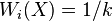 if is among the
  closest points to in
  and
and  otherwise.
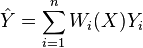
Random forests with constant leaf predictors can be interpreted as a weighted neighborhood scheme in the following way. Given a forest of  trees, the prediction that the
  -th tree makes for can be written as
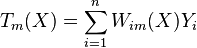
where  is equal to
  if and are in the same leaf in the -th tree and otherwise, and
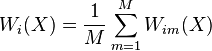
  is the number of training data which fall in the same leaf as in the -th tree. The prediction of the whole forest is

which shows that the random forest prediction is a weighted average of the  's, with weights
The neighbors of in this interpretation are the points which fall in the same leaf as in at least one tree of the forest. In this way, the neighborhood of depends in a complex way on the structure of the trees, and thus on the structure of the training set.
This connection was first described by Lin and Jeon in a technical report from 2001[9] where they show that the shape of the neighborhood used by a random forest adapts to the local importance of each feature.
Variable Importance[edit]
Random forests can be used to rank the importance of variables in a regression or classification problem in a natural way. The following technique was described Breiman's original paper[1] and is implemented in the R package randomForest.[2]
The first step in measuring the variable importance in a data set is to fit a random forest to the data. During the fitting process the out-of-bag error for each data point is recorded and averaged over the forest (errors on an independent test set can be substituted if bagging is not used during training).
To measure the importance of the  -th feature after training, the values of the -th feature are permuted among the training data and the out-of-bag error is again computed on this perturbed data set. The importance score for the -th feature is computed by averaging the difference in out-of-bag error before and after the permutation over all trees. The score is normalized by the standard deviation of these differences.
Features which produce large values for this score are ranked as more important than features which produce small values.
This method of determining variable importance has some drawbacks. For data including categorical variables with different number of levels, random forests are biased in favor of those attributes with more levels. Methods such as partial permutations can be used to solve the problem.[10][11] If the data contain groups of correlated features of similar relevance for the output, then smaller groups are favored over larger groups.[12]
See also[edit]
References[edit]
- ^ Jump up to:a b c Breiman, Leo (2001). "Random Forests". Machine Learning 45 (1): 5–32. doi:10.1023/A:1010933404324.
- ^ Jump up to:a b Liaw, Andy (16 October 2012). "Documentation for R package randomForest". Retrieved 15 March 2013.
- Jump up^ Ho, Tin Kam (1995). "Random Decision Forest". Proceedings of the 3rd International Conference on Document Analysis and Recognition, Montreal, QC, 14–16 August 1995. pp. 278–282.
- ^ Jump up to:a b Ho, Tin Kam (1998). "The Random Subspace Method for Constructing Decision Forests". IEEE Transactions on Pattern Analysis and Machine Intelligence 20 (8): 832–844. doi:10.1109/34.709601.
- ^ Jump up to:a b Amit, Yali; Geman, Donald (1997). "Shape quantization and recognition with randomized trees". Neural Computation 9 (7): 1545–1588. doi:10.1162/neco.1997.9.7.1545.
- Jump up^ Kleinberg, Eugene (1996). "An Overtraining-Resistant Stochastic Modeling Method for Pattern Recognition". Annals of Statistics 24 (6): 2319–2349. doi:10.1214/aos/1032181157. MR 1425956.
- Jump up^ Dietterich, Thomas (2000). "An Experimental Comparison of Three Methods for Constructing Ensembles of Decision Trees: Bagging, Boosting, and Randomization". Machine Learning: 139–157.
- ^ Jump up to:a b Criminisi, Antonio; Shotton, Jamie; Konukoglu, Ender (2011). "Decision Forests: A Unified Framework for Classification, Regression, Density Estimation, Manifold Learning and Semi-Supervised Learning". Foundations and Trends in Computer Vision 7: 81–227. doi:10.1561/0600000035.
- Jump up^ Lin, Yi; Jeon, Yongho (2002), "Random forests and adaptive nearest neighbors", Technical Report No. 1055, University of Wisconsin
- Jump up^ Deng,H.; Runger, G.; Tuv, E. (2011). "Bias of importance measures for multi-valued attributes and solutions". Proceedings of the 21st International Conference on Artificial Neural Networks (ICANN). pp. 293–300.
- Jump up^ Altmann A, Tolosi L, Sander O, Lengauer T (2010). "Permutation importance:a corrected feature importance measure".Bioinformatics. doi:10.1093/bioinformatics/btq134.
- Jump up^ Tolosi L, Lengauer T (2011). "Classification with correlated features: unreliability of feature ranking and solutions.".Bioinformatics. doi:10.1093/bioinformatics/btr300.
External links[edit]
- Random Forests classifier description (Site of Leo Breiman)
- Liaw, Andy & Wiener, Matthew "Classification and Regression by randomForest" R News (2002) Vol. 2/3 p. 18(Discussion of the use of the random forest package for R)
- Ho, Tin Kam (2002). "A Data Complexity Analysis of Comparative Advantages of Decision Forest Constructors". Pattern Analysis and Applications 5, p. 102-112 (Comparison of bagging and random subspace method)
- Prinzie, Anita; Poel, Dirk (2007). "Random Multiclass Classification: Generalizing Random Forests to Random MNL and Random NB". Database and Expert Systems Applications. Lecture Notes in Computer Science 4653. p. 349.doi:10.1007/978-3-540-74469-6_35. ISBN 978-3-540-74467-2.
- Prinzie, Anita; Van Den Poel, Dirk (2008). "Random Forests for multiclass classification: Random MultiNomial Logit".Expert Systems with Applications 34 (3): 1721. doi:10.1016/j.eswa.2007.01.029.
- C# implementation of random forest algorithm for categorization of text documents supporting reading of documents, making dictionaries, filtering stop words, stemming, counting words, making document-term matrix and its usage for building random forest and further categorization.
- A python implementation of the random forest algorithm working in regression, classification with multi-output support.
- RFTK is a flexible toolkit for building random forests with python bindings.