FastICA is an efficient and popular algorithm for independent component analysis invented by Aapo Hyvärinen at Helsinki University of Technology. The algorithm is based on a fixed-point iteration scheme maximizing non-Gaussianity as a measure ofstatistical independence. It can also be derived as an approximative Newton iteration.
Contents
[hide] - 1 Algorithm
- 1.1 Preprocess the data
- 1.1.1 Centering the data
- 1.1.2 Whitening the data
- 1.2 Single component extraction
- 1.3 Multiple component extraction
- 2 See also
- 3 References
- 4 External links
Algorithm[edit]
Preprocess the data[edit]
Before the FastICA algorithm can be applied, the input vector data  should be centered and whitened.
Centering the data[edit]
The input data is centered by computing the mean of each component of and subtracting that mean. This has the effect of making each component have zero mean. Thus:
Whitening the data[edit]
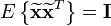
Whitening the data involves linearly transforming the data so that the new components are uncorrelated and have variance one. If  is the whitened data, then the covariance matrix of the whitened data is the identity matrix:
This can be done using eigenvalue decomposition of the covariance matrix of the data:  , where
  is the matrix of eigenvectors and
  is the diagonal matrix of eigenvalues. Once eigenvalue decomposition is done, the whitened data is:

The iterative algorithm finds the direction for the weight vector  maximizing the non-Gaussianity of the projection
  for the data . The function
  is the derivative of a nonquadratic nonlinearity function
  . Hyvärinen states that good equations for
  (shown with their derivatives
  and second derivatives
  ) are:
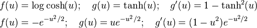
The first equation is a good general-purpose equation, while the second is highly robust.
- Randomize the initial weight vector
- Let
 , where
  means averaging over all column-vectors of matrix
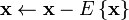
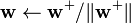
- Let
- If not converged, go back to 2
The single unit iterative algorithm only estimates one of the independent components, to estimate more the algorithm must repeated, and the projection vectors decorated. Although Hyvärinen provides several ways of decorating results the simplest multiple unit algorithm follows.  indicates a column vector of 1's with dimension M.
Algorithm FastICA
- Input:
 Number of desired components
 - Input:
 Matrix, where each column represents an N-dimensional sample, where
- Output:
 Un-mixing matrix where each row projects X onto into independent component.
 - Output:
 Independent components matrix, with M columns representing a sample with C dimensions.
for p in 1 to C:  Random vector of length N while
  changes
 Output:
  Output:
See also[edit]
References[edit]
External links[edit]