Diffusion maps is a machine learning algorithm introduced by R. R. Coifman and S. Lafon.[1][2] It computes a family of embeddings of a data set into Euclidean space (often low-dimensional) whose coordinates can be computed from the eigenvectors and eigenvalues of a diffusion operator on the data. The Euclidean distance between points in the embedded space is equal to the "diffusion distance" between probability distributions centered at those points. Different from other dimensionality reduction methods such as principal component analysis (PCA) and multi-dimensional scaling (MDS), diffusion maps is a non-linear method that focuses on discovering the underlying manifold that the data has been sampled from. By integrating local similarities at different scales, diffusion maps gives a global description of the data-set. Compared with other methods, the diffusion maps algorithm is robust to noise perturbation and is computationally inexpensive.
Contents
[hide] - 1 Definition of diffusion maps
- 1.1 Connectivity
- 1.2 Diffusion process
- 1.3 Diffusion distance
- 1.4 Diffusion process
- 2 Algorithm
- 3 Application
- 4 See also
- 5 References
Definition of diffusion maps[edit]
Following,[3] diffusion maps can be defined in four steps.
Connectivity[edit]
Diffusion maps leverages the relationship between heat diffusion and random walk Markov chain. The basic observation is that if we take a random walk on the data, walking to a nearby data-point is more likely than walking to another that is far away. Based on this, the connectivity between two data points,  and
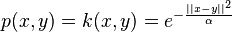
and  , can be defined as the probability of walking from to in one step of the random walk. Usually, this probability will be defined as the kernel function on the two points, for example, the popular Gaussian kernel:
More generally, the kernel function has the following properties
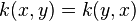
( is symmetric)
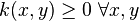
( is positivity preserving).
The kernel constitutes the prior definition of the local geometry of data-set. Since a given kernel will capture a specific feature of the data set, its choice should be guided by the application that one has in mind.
Diffusion process[edit]
With the definition of connectivity between two points, we can define the diffusion matrix  (it is also a version of graph Laplacian matrix)
Many works use the normalized matrix as

We can define the probabilities for taken from  to
to  in
in  steps as:

As we calculate the probabilities for increasing values of , we observe the data-set at different scales. This is the diffusion process. Diffusion process reveals the global geometric structure of a data set as paths along the true geometric structure of the data set have high probability.
Diffusion distance[edit]
The diffusion distance at time between two points can be measured as the similarity of two points in the observation space with the connectivity between them. It is given by
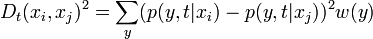
here  is a weighted function which can often treated as
Diffusion process[edit]
Now, we can give the definition of diffusion map as:

in,[4] it is proved that

if we take the first k eigenvectors and eigenvalues, we get the diffusion map from the original data to a k-dimensional space which is embedded in the original space.
Algorithm[edit]
The basic algorithm framework of diffusion map is as:
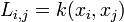
Step 1. Given the similarity matrix L
Step 2. Form the normalized matrix 
Step 3. Compute the k largest eigenvalues of  and the corresponding eigenvectors
Step 4. Use diffusion map to get the embedding matrix Y
Application[edit]
In the paper,[4] they showed how to design a kernel that reproduces the diffusion induced by a Fokker-Planck equation. Also, they explained that when the data approximate a manifold, then one can recover the geometry of this manifold by computing an approximation of the Laplace-Beltrami operator. This computation is completely insensitive to the distribution of the points and therefore provides a separation of the statistics and the geometry of the data. Since Diffusion map gives a global description of the data-set, it can measure the distances between pair of sample points in the manifold the data is embedded. Based on diffusion map, there are many applications, such as spectral clustering, low dimensional representation of images, image segmentation,[5]3D model segmentation,[6] speaker identification,[7] sampling on manifolds and so on.
See also[edit]
References[edit]
- ^ Coifman, R.R.; S. Lafon. (2006). "Diffusion maps". Applied and Computational Harmonic Analysis.
- ^ Lafon, S.S. (2004). "Diffusion Maps and Geometric Harmonics". PhD thesis, Yale University.
- ^ J De, Porte; B M; Hereman, W; Walt, S J Van Der (2008). "An Introduction to Diffusion Maps". Techniques.
- ^ a b Nadler, Boaz; Stéphane Lafon ; Ronald R. Coifman ; Ioannis G. Kevrekidis (2005). "Diffusion Maps, Spectral Clustering and Eigenfunctions of Fokker–Planck Operators". in Advances in Neural Information Processing Systems 18.
- ^ Zeev, Farbman; Fattal Raanan ;Lischinski Dani (2010). "Diffusion maps for edge-aware image editing". ACM Trans. Graph 29: 145:1–145:10.
- ^ Oana, Sidi; Oliver van Kaick ; Yanir Kleiman ; Hao Zhang ; Daniel Cohen-Or (2011). "Unsupervised Co-Segmentation of a Set of Shapes via Descriptor-Space Spectral Clustering". ACM Transactions on Graphics.
- ^ Michalevsky, Yan; Ronen Talmon ; Israel Cohen (2011). Speaker Identification Using Diffusion Maps. European signal processing conference 2011.