In statistics and machine learning, a Bayesian interpretation of regularization for kernel methods is often useful. Kernel methods are central to both the regularization and the Bayesian point of views in machine learning. In regularization they are a natural choice for the hypothesis space and the regularization functional through the notion of reproducing kernel Hilbert spaces. In Bayesian probability they are a key component of Gaussian processes, where the kernel function is known as the covariance function. Kernel methods have traditionally been used in supervised learning problems where the input space is usually a space of vectors while the output space is a space of scalars. More recently these methods have been extended to problems that deal with multiple outputs such as in multi-task learning.[1]
In this article we analyze the connections between the regularization and Bayesian point of views for kernel methods in the case of scalar outputs. A mathematical equivalence between the regularization and the Bayesian point of views is easily proved in cases where the reproducing kernel Hilbert space is finite-dimensional. The infinite-dimensional case raises subtle mathematical issues; we will consider here the finite-dimensional case. We start with a brief review of the main ideas underlying kernel methods for scalar learning, and briefly introduce the concepts of regularization and Gaussian processes. We then show how both point of views arrive at essentially equivalent estimators, and show the connection that ties them together.
Contents
[hide] - 1 The Supervised Learning Problem
- 2 A Regularization Perspective
- 2.1 Reproducing Kernel Hilbert Space
- 2.2 The Regularized Functional
- 2.3 Derivation of the Estimator
- 3 A Bayesian Perspective
- 3.1 A Review of Bayesian Probability
- 3.2 The Gaussian Process
- 3.3 Derivation of the Estimator
- 4 The Connection Between Regularization and Bayes
- 5 References
The Supervised Learning Problem[edit]
The classical supervised learning problem requires estimating the output for some new input point  by learning a scalar-valued estimator
  on the basis of a training set
  consisting of
  input-output pairs,
  .[2][3][4] Given a symmetric and positive bivariate function
  called a kernel, one of the most popular estimators in machine learning is given by
-
where  is the kernel matrix with entries
  ,
, ![\mathbf{k} = [k(\mathbf{x}_1,\mathbf{x}'),\ldots,k(\mathbf{x}_n,\mathbf{x}')]^\top](http://upload.wikimedia.org/math/2/8/1/2818904d82a2e6cc8fd4c188e7e69b4b.png) , and
, and ![\mathbf{Y} = [y_1,\ldots,y_n]^\top](http://upload.wikimedia.org/math/6/f/3/6f3544ab1671fc3fde221d7c34786642.png) . We will see how this estimator can be derived both from a regularization and a Bayesian perspective.
. We will see how this estimator can be derived both from a regularization and a Bayesian perspective.
A Regularization Perspective[edit]
The main assumption in the regularization perspective is that the set of functions  is assumed to belong to a reproducing kernel Hilbert space
  .[2][5][6][7]
Reproducing Kernel Hilbert Space[edit]
A reproducing kernel Hilbert space (RKHS) is a Hilbert space of functions defined by a symmetric, positive-definite function  called the reproducing kernel such that the function
  belongs to for all
  .[8][9][10] There are three main properties make an RKHS appealing:
1. The reproducing property, which gives name to the space,

where  is the inner product in .
2. Functions in an RKHS are in the closure of the linear combination of the kernel at given points,
 .
.
This allows the construction in a unified framework of both linear and generalized linear models.
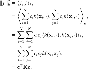
3. The norm in an RKHS can be written as
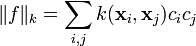
and is a natural measure of how complex the function is.
The Regularized Functional[edit]
The estimator is derived as the minimizer of the regularized functional
-
where  and
and  is the norm in . The first term in this functional, which measures the average of the squares of the errors between the
  and the
  , is called the empirical risk and represents the cost we pay by predicting for the true value . The second term in the functional is the squared norm in a RKHS multiplied by a weight
  and serves the purpose of stabilizing the problem[5][7] as well as of adding a trade-off between fitting and complexity of the estimator.[2] The weight , called the regularizer, determines the degree to which instability and complexity of the estimator should be penalized (higher penalty for increasing value of ).
Derivation of the Estimator[edit]
The explicit form of the estimator in equation (1) is derived in two steps. First, the representer theorem[11][12][13] states that the minimizer of the functional (2) can always be written as a linear combination of the kernels centered at the training-set points,
-
for some  . The explicit form of the coefficients
 ![\mathbf{c} = [c_1,\ldots,c_n]^\top](http://upload.wikimedia.org/math/5/b/e/5be33edae46aa6cdd59cac48d64859f0.png) can be found by substituting for
can be found by substituting for  in the functional (2). For a function of the form in equation (3), we have that
We can rewrite the functional (2) as
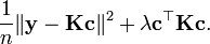
This functional is convex in  and therefore we can find its minimum by setting the gradient with respect to to zero,
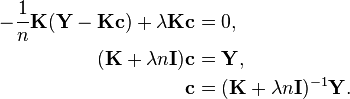
Substituting this expression for the coefficients in equation (3), we obtain the estimator stated previously in equation (1),
A Bayesian Perspective[edit]
The notion of a kernel plays a crucial role in Bayesian probability as the covariance function of a stochastic process called the Gaussian process.
A Review of Bayesian Probability[edit]
As part of the Bayesian framework, the Gaussian process specifies the prior distribution that describes the prior beliefs about the properties of the function being modeled. These beliefs are updated after taking into account observational data by means of alikelihood function that relates the prior beliefs to the observations. Taken together, the prior and likelihood lead to an updated distribution called the posterior distribution that is customarily used for predicting test cases.
The Gaussian Process[edit]
A Gaussian process (GP) is a stochastic process in which any finite number of random variables that are sampled follow a joint Normal distribution.[14] The mean vector and covariance matrix of the Gaussian distribution completely specify the GP. GPs are usually used as a priori distribution for functions, and as such the mean vector and covariance matrix can be viewed as functions, where the covariance function is also called the kernel of the GP. Let a function  follow a Gaussian process with mean function
  and kernel function
  ,
,
In terms of the underlying Gaussian distribution, we have that for any finite set  if we let
 ![f(\mathbf{X}) = [f(\mathbf{x}_1),\ldots,f(\mathbf{x}_n)]^\top](http://upload.wikimedia.org/math/9/8/1/9812a20d16154759c41b90bb65920761.png) then
then
where ![\mathbf{m} = m(\mathbf{X}) = [m(\mathbf{x}_1),\ldots,m(\mathbf{x}_N)]^\top](http://upload.wikimedia.org/math/b/6/f/b6faf3538a5546d6f7484e586eb3b85b.png) is the mean vector and
is the mean vector and 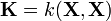 is the covariance matrix of the multivariate Gaussian distribution.
Derivation of the Estimator[edit]
In a regression context, the likelihood function is usually assumed to be a Gaussian distribution and the observations to be independent and identically distributed (iid),

This assumption corresponds to the observations being corrupted with zero-mean Gaussian noise with variance  . The iid assumption makes it possible to factorize the likelihood function over the data points given the set of inputs
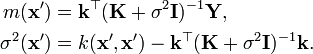
  and the variance of the noise , and thus the posterior distribution can be computed analytically. For a test input vector , given the training data
 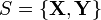 , the posterior distribution is given by

where  denotes the set of parameters which include the variance of the noise and any parameters from the covariance function and where
The Connection Between Regularization and Bayes[edit]
A connection between regularization theory and Bayesian theory can only be achieved in the case of finite dimensional RKHS. Under this assumption, regularization theory and Bayesian theory are connected through Gaussian process prediction.[5][14]
In the finite dimensional case, every RKHS can be described in terms of a feature map  such that[2]
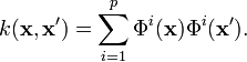
Functions in the RKHS with kernel  can be then be written as
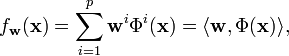
and we also have that
We can now build a Gaussian process by assuming ![\mathbf{w} = [w^1,\ldots,w^p]^\top](http://upload.wikimedia.org/math/f/2/2/f2299214b0833f6660e0b3e1033e6852.png) to be distributed according to a multivariate Gaussian distribution with zero mean and identity covariance matrix,
to be distributed according to a multivariate Gaussian distribution with zero mean and identity covariance matrix,

If we assume a Gaussian likelihood we have

where  . The resulting posterior distribution is the given by
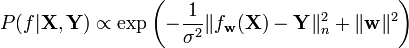
We can see that a maximum posterior (MAP) estimate is equivalent to the minimization problem defining Tikhonov regularization, where in the Bayesian case the regularization parameter is related to the noise variance.
From a philosophical perspective, the loss function in a regularization setting plays a different role than the likelihood function in the Bayesian setting. Whereas the loss function measures the error that is incurred when predicting  in place of
  , the likelihood function measures how likely the observations are from the model that was assumed to be true in the generative process. From a mathematical perspective, however, the formulations of the regularization and Bayesian frameworks make the loss function and the likelihood function to have the same mathematical role of promoting the inference of functions that approximate the labels as much as possible.
References[edit]
- Jump up^ Álvarez, Mauricio A.; Rosasco, Lorenzo; Lawrence, Neil D. (June 2011). "Kernels for Vector-Valued Functions: A Review". ArXiv e-prints.
- ^ Jump up to:a b c d Vapnik, Vladimir (1998). Statistical learning theory. Wiley. ISBN 9780471030034.
- Jump up^ Hastie, Trevor; Tibshirani, Robert; Friedman, Jerome H. (2009). The Elements of Statistical Learning: Data Mining, Inference and Prediction (2, illustrated ed.). Springer. ISBN 9780387848570.
- Jump up^ Bishop, Christopher M. (2009). Pattern recognition and machine learning. Springer. ISBN 9780387310732.
- ^ Jump up to:a b c Wahba, Grace (1990). Spline models for observational data. SIAM.
- Jump up^ Schölkopf, Bernhard; Smola, Alexander J. (2002). Learning with Kernels: Support Vector Machines, Regularization, Optimization, and Beyond. MIT Press. ISBN 9780262194754.
- ^ Jump up to:a b Girosi, F.; Poggio, T. (1990). "Networks and the best approximation property". Biological Cybernetics (Springer) 63 (3): 169–176.
- Jump up^ Aronszajn, N (May 1950). "Theory of Reproducing Kernels". Transactions of the American Mathematical Society 68 (3): 337–404.
- Jump up^ Schwartz, Laurent (1964). "Sous-espaces hilbertiens d’espaces vectoriels topologiques et noyaux associés (noyaux reproduisants)". Journal d'analyse mathématique (Springer) 13 (1): 115–256.
- Jump up^ Cucker, Felipe; Smale, Steve (October 5, 2001). "On the mathematical foundations of learning". Bulletin of the American Mathematical Society 39 (1): 1–49.
- Jump up^ Kimeldorf, George S.; Wahba, Grace (1970). "A correspondence between Bayesian estimation on stochastic processes and smoothing by splines". The Annals of Mathematical Statistics 41 (2): 495–502. doi:10.1214/aoms/1177697089.
- Jump up^ Schölkopf, Bernhard; Herbrich, Ralf; Smola, Alex J. (2001). "A Generalized Representer Theorem". COLT/EuroCOLT 2001, LNCS. 2111/2001: 416–426. doi:10.1007/3-540-44581-1_27.
- Jump up^ De Vito, Ernesto; Rosasco, Lorenzo; Caponnetto, Andrea; Piana, Michele; Verri, Alessandro (October 2004). "Some Properties of Regularized Kernel Methods". Journal of Machine Learning Research 5: 1363–1390.
- ^ Jump up to:a b Rasmussen, Carl Edward; Williams, Christopher K. I. (2006). Gaussian Processes for Machine Learning. The MIT Press. ISBN 0-262-18253-X.