
A graphical representation of an example Boltzmann machine. Each undirected edge represents dependency. In this example there are 3 hidden units and 4 visible units. This is not a restricted Boltzmann machine.
A Boltzmann machine is a type of stochastic recurrent neural network invented by Geoffrey Hinton and Terry Sejnowski in 1985. Boltzmann machines can be seen as the stochastic, generativecounterpart of Hopfield nets. They were one of the first examples of a neural network capable of learning internal representations, and are able to represent and (given sufficient time) solve difficult combinatoric problems. However, due to a number of issues discussed below, Boltzmann machines with unconstrained connectivity have not proven useful for practical problems in machine learning or inference. They are still theoretically intriguing, however, due to the locality and Hebbian nature of their training algorithm, as well as their parallelism and the resemblance of their dynamics to simple physical processes. If the connectivity is constrained, the learning can be made efficient enough to be useful for practical problems.
They are named after the Boltzmann distribution in statistical mechanics, which is used in their sampling function.
Structure[edit]

A graphical representation of a Boltzmann machine with a few weights labeled. Each undirected edge represents dependency and is weighted with weight

. In this example there are 3 hidden units (blue) and 4 visible units (white). This is not a restricted Boltzmann machine.
A Boltzmann machine, like a Hopfield network, is a network of units with an "energy" defined for the network. It also has binary units, but unlike Hopfield nets, Boltzmann machine units arestochastic. The global energy,  , in a Boltzmann machine is identical in form to that of a Hopfield network:

Where:
- is the connection strength between unit
 and unit
  .
.  is the state,
  , of unit .
 is the bias of unit in the global energy function. (
 is the activation threshold for the unit.)
The connections in a Boltzmann machine have two restrictions:
 . (No unit has a connection with itself.)
 . (All connections are symmetric.)
Often the weights are represented in matrix form with a symmetric matrix  , with zeros along the diagonal.
Probability of a unit's state[edit]
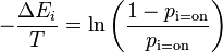
The difference in the global energy that results from a single unit being 0 (off) versus 1 (on), written  , is given by:

This can be expressed as the difference of energies of two states:
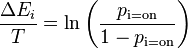
We then substitute the energy of each state with its relative probability according to the Boltzmann Factor (the property of a Boltzmann distribution that the energy of a state is proportional to the negative log probability of that state):

where  is Boltzmann's constant and is absorbed into the artificial notion of temperature
  . We then rearrange terms and consider that the probabilities of the unit being on and off must sum to one:


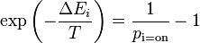
We can now finally solve for  , the probability that the -th unit is on.

where the scalar is referred to as the temperature of the system. This relation is the source of the logistic function found in probability expressions in variants of the Boltzmann machine.
Equilibrium state[edit]
The network is run by repeatedly choosing a unit and setting its state according to the above formula. After running for long enough at a certain temperature, the probability of a global state of the network will depend only upon that global state's energy, according to a Boltzmann distribution. This means that log-probabilities of global states become linear in their energies. This relationship is true when the machine is "at thermal equilibrium", meaning that the probability distribution of global states has converged. If we start running the network from a high temperature, and gradually decrease it until we reach a thermal equilibrium at a low temperature, we may converge to a distribution where the energy level fluctuates around the global minimum.[citation needed] This process is called simulated annealing.
If we want to train the network so that the chance it will converge to a global state is according to an external distribution that we have over these states, we need to set the weights so that the global states with the highest probabilities will get the lowest energies. This is done by the following training procedure.
Training[edit]
The units in the Boltzmann Machine are divided into "visible" units, V, and "hidden" units, H. The visible units are those, which receive information from the "environment", i.e. our training set is a set of binary vectors over the set V. The distribution over the training set is denoted  .
.
As is discussed above, the distribution over global states converges as the Boltzmann machine reaches thermal equilibrium. We denote this distribution, after we marginalize it over the hidden units, as  .
.
Our goal is to approximate the "real" distribution using the which will be produced (eventually) by the machine. To measure how similar the two distributions are, we use the Kullback-Leibler divergence,  :
:

where the sum is over all the possible states of  . is a function of the weights, since they determine the energy of a state, and the energy determines
  , as promised by the Boltzmann distribution. Hence, we can use agradient descent algorithm over , so a given weight, is changed by subtracting the partial derivative of with respect to the weight.
There are two phases to Boltzmann machine training, and we switch iteratively between them. One is the "positive" phase where the visible units' states are clamped to a particular binary state vector sampled from the training set (according to  ). The other is the "negative" phase where the network is allowed to run freely, i.e. no units have their state determined by external data. Surprisingly enough, the gradient with respect to a given weight, , is given by the very simple equation (proved in Ackley et al.[1]):
![\frac{\partial{G}}{\partial{w_{ij}}} = -\frac{1}{R}[p_{ij}^{+}-p_{ij}^{-}]](http://upload.wikimedia.org/math/6/e/1/6e1526c4fba6e2d2466ab7816e3dc651.png)
where:
 is the probability of units i and j both being on when the machine is at equilibrium on the positive phase.
 is the probability of units i and j both being on when the machine is at equilibrium on the negative phase.
 denotes the learning rate
This result follows from the fact that at thermal equilibrium the probability  of any global state
  when the network is free-running is given by the Boltzmann distribution (hence the name "Boltzmann machine").
Remarkably, this learning rule is fairly biologically plausible because the only information needed to change the weights is provided by "local" information. That is, the connection (or synapse biologically speaking) does not need information about anything other than the two neurons it connects. This is far more biologically realistic than the information needed by a connection in many other neural network training algorithms, such as backpropagation.
The training of a Boltzmann machine does not use the EM algorithm, which is heavily used in machine learning. By minimizing the KL-divergence, it is equivalent as maximizing the log-likelihood of the data. Therefore, the training procedure performs gradient ascent on the log-likelihood of the observed data. This is in contrast to the EM algorithm, where the posterior distribution of the hidden nodes must be calculated before the maximization of the expected value of the complete data likelihood during the M-step.
Training the biases is similar, but uses only single node activity:
![\frac{\partial{G}}{\partial{\theta_{i}}} = -\frac{1}{R}[p_{i}^{+}-p_{i}^{-}]](http://upload.wikimedia.org/math/b/d/5/bd56720c20762eabad6fe8cbe03fdd83.png)
Problems[edit]
The Boltzmann machine would theoretically be a rather general computational medium. For instance, if trained on photographs, the machine would theoretically model the distribution of photographs, and could use that model to, for example, complete a partial photograph.
Unfortunately, there is a serious practical problem with the Boltzmann machine, namely that the learning seems to stop working correctly when the machine is scaled up to anything larger than a trivial machine.[citation needed] This is due to a number of effects, the most important of which are:
- the time the machine must be run in order to collect equilibrium statistics grows exponentially with the machine's size, and with the magnitude of the connection strengths
- connection strengths are more plastic when the units being connected have activation probabilities intermediate between zero and one, leading to a so-called variance trap. The net effect is that noise causes the connection strengths to random walk until the activities saturate.
Restricted Boltzmann machine[edit]
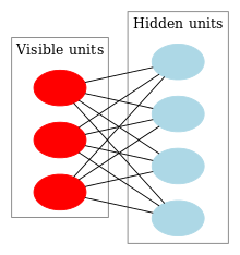
Graphical representation of a restricted Boltzmann machine. The four blue units represent hidden units, and the three red units represent visible states. In restricted Boltzmann machines there are only connections (dependencies) between hidden and visible units, and none between units of the same type (no hidden-hidden, nor visible-visible connections).
Although learning is impractical in general Boltzmann machines, it can be made quite efficient in an architecture called the "restricted Boltzmann machine" or "RBM" which does not allow intralayer connections between hidden units. After training one RBM, the activities of its hidden units can be treated as data for training a higher-level RBM. This method of stacking RBM's makes it possible to train many layers of hidden units efficiently and is one of the most common deep learning strategies. As each new layer is added the overall generative model gets better.
There is an extension to the restricted Boltzmann machine that affords using real valued data rather than binary data. Along with higher order Boltzmann machines, it is outlined here [1].
One example of a practical application of Restricted Boltzmann machines is the performance improvement of speech recognition software.[2]
History[edit]
The Boltzmann machine is a Monte Carlo version of the Hopfield network.
The idea of using annealed Ising models for inference is often thought to have been first described by:
- Geoffrey E. Hinton and Terrence J. Sejnowski, Analyzing Cooperative Computation. In Proceedings of the 5th Annual Congress of the Cognitive Science Society, Rochester, NY, May 1983.
- Geoffrey E. Hinton and Terrence J. Sejnowski, Optimal Perceptual Inference. In Proceedings of the IEEE conference on Computer Vision and Pattern Recognition (CVPR), pages 448–453, IEEE Computer Society, Washington DC, June 1983.
However, it should be noted that these articles appeared after the seminal publication by John Hopfield, where the connection to physics and statistical mechanics was made in the first place, mentioning spin glasses:
- John J. Hopfield, Neural networks and physical systems with emergent collective computational abilities, Proc. Natl. Acad. Sci. USA, vol. 79 no. 8, pp. 2554-2558, April 1982.
The idea of applying the Ising model with annealed Gibbs sampling is also present in Douglas Hofstadter's Copycat project:
- Hofstadter, Douglas R., The Copycat Project: An Experiment in Nondeterminism and Creative Analogies. MIT Artificial Intelligence Laboratory Memo No. 755, January 1984.
- Hofstadter, Douglas R., A Non-Deterministic Approach to Analogy, Involving the Ising Model of Ferromagnetism. In E. Caianiello, ed. The Physics of Cognitive Processes. Teaneck, NJ: World Scientific, 1987.
Similar ideas (with a change of sign in the energy function) are also found in Paul Smolensky's "Harmony Theory".
The explicit analogy drawn with statistical mechanics in the Boltzmann Machine formulation led to the use of terminology borrowed from physics (e.g., "energy" rather than "harmony"), which has become standard in the field. The widespread adoption of this terminology may have been encouraged by the fact that its use led to the importation of a variety of concepts and methods from statistical mechanics. However, there is no reason to think that the various proposals to use simulated annealing for inference described above were not independent. (Helmholtz made a similar analogy during the dawn of psychophysics.)
Ising models are now considered to be a special case of Markov random fields, which find widespread application in various fields, including linguistics, robotics, computer vision, and artificial intelligence.
See also[edit]
derived from the reversed form of ,
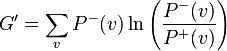 .
.
References[edit]
Further reading[edit]
External links[edit]