In the field of mathematical modeling, a radial basis function network is an artificial neural network that uses radial basis functions as activation functions. The output of the network is a linear combination of radial basis functions of the inputs and neuron parameters. Radial basis function networks have many uses, including function approximation, time series prediction, classification, and system control. They were first formulated in a 1988 paper by Broomhead and Lowe, both researchers at the Royal Signals and Radar Establishment.[1][2][3]
Network architecture[edit]

Figure 1: Architecture of a radial basis function network. An input vector
x is used as input to all radial basis functions, each with different parameters. The output of the network is a linear combination of the outputs from radial basis functions.
Radial basis function (RBF) networks typically have three layers: an input layer, a hidden layer with a non-linear RBF activation function and a linear output layer. The input can be modeled as a vector of real numbers  . The output of the network is then a scalar function of the input vector,
  , and is given by
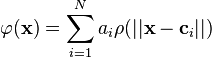
where N is the number of neurons in the hidden layer,  is the center vector for neuron i, and
  is the weight of neuron i in the linear output neuron. Functions that depend only on the distance from a center vector are radially symmetric about that vector, hence the name radial basis function. In the basic form all inputs are connected to each hidden neuron. The norm is typically taken to be the Euclidean distance (although theMahalanobis distance appears to perform better in general) and the radial basis function is commonly taken to be Gaussian
![\rho \big ( \left \Vert \mathbf{x} - \mathbf{c}_i \right \Vert \big ) = \exp \left[ -\beta \left \Vert \mathbf{x} - \mathbf{c}_i \right \Vert ^2 \right]](http://upload.wikimedia.org/math/c/a/8/ca850699487e278678e96a1d0da23f22.png) .
.
The Gaussian basis functions are local to the center vector in the sense that

i.e. changing parameters of one neuron has only a small effect for input values that are far away from the center of that neuron.
Given certain mild conditions on the shape of the activation function, RBF networks are universal approximators on acompact subset of  . [4] This means that an RBF network with enough hidden neurons can approximate any continuous function with arbitrary precision.
The parameters ,  , and
, and  are determined in a manner that optimizes the fit between
  and the data.

Figure 2: Two unnormalized radial basis functions in one input dimension. The basis function centers are located at

and

.
Normalized[edit]
Normalized architecture[edit]
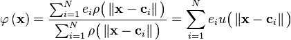
In addition to the above unnormalized architecture, RBF networks can be normalized. In this case the mapping is

where
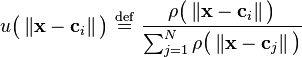
is known as a "normalized radial basis function".

Figure 3: Two normalized radial basis functions in one input dimension. The basis function centers are located at
and
.
Theoretical motivation for normalization[edit]
There is theoretical justification for this architecture in the case of stochastic data flow. Assume a stochastic kernel approximation for the joint probability density

where the weights and  are exemplars from the data and we require the kernels to be normalized
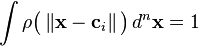
and
 .
.

Figure 4: Three normalized radial basis functions in one input dimension. The additional basis function has center at

The probability densities in the input and output spaces are

and
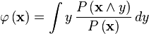
The expectation of y given an input  is
is

where

is the conditional probability of y given . The conditional probability is related to the joint probability through Bayes theorem

which yields
 .
.
This becomes
when the integrations are performed.

Figure 5: Four normalized radial basis functions in one input dimension. The fourth basis function has center at

. Note that the first basis function (dark blue) has become localized.
Local linear models[edit]
It is sometimes convenient to expand the architecture to include local linear models. In that case the architectures become, to first order,
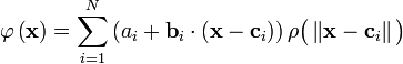
and

in the unnormalized and normalized cases, respectively. Here  are weights to be determined. Higher order linear terms are also possible.
This result can be written

where
![e_{ij} = \begin{cases} a_i, & \mbox{if } i \in [1,N] \\ b_{ij}, & \mbox{if }i \in [N+1,2N] \end{cases}](http://upload.wikimedia.org/math/9/d/5/9d552af93ae3310da493d4e7133586bf.png)
and
![v_{ij}\big ( \mathbf{x} - \mathbf{c}_i \big ) \ \stackrel{\mathrm{def}}{=}\ \begin{cases} \delta_{ij} \rho \big ( \left \Vert \mathbf{x} - \mathbf{c}_i \right \Vert \big ) , & \mbox{if } i \in [1,N] \\ \left ( x_{ij} - c_{ij} \right ) \rho \big ( \left \Vert \mathbf{x} - \mathbf{c}_i \right \Vert \big ) , & \mbox{if }i \in [N+1,2N] \end{cases}](http://upload.wikimedia.org/math/8/b/c/8bca67d51c43112c90b95fed8b871f35.png)
in the unnormalized case and
![v_{ij}\big ( \mathbf{x} - \mathbf{c}_i \big ) \ \stackrel{\mathrm{def}}{=}\ \begin{cases} \delta_{ij} u \big ( \left \Vert \mathbf{x} - \mathbf{c}_i \right \Vert \big ) , & \mbox{if } i \in [1,N] \\ \left ( x_{ij} - c_{ij} \right ) u \big ( \left \Vert \mathbf{x} - \mathbf{c}_i \right \Vert \big ) , & \mbox{if }i \in [N+1,2N] \end{cases}](http://upload.wikimedia.org/math/0/7/7/077c4c4d82db1a37647bd41061d69287.png)
in the normalized case.
Here  is a Kronecker delta function defined as
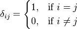 .
.
Training[edit]
RBF networks are typically trained by a two-step algorithm. In the first step, the center vectors of the RBF functions in the hidden layer are chosen. This step can be performed in several ways; centers can be randomly sampled from some set of examples, or they can be determined using k-means clustering. Note that this step is unsupervised. A thirdbackpropagation step can be performed to fine-tune all of the RBF net's parameters.[3]
The second step simply fits a linear model with coefficients  to the hidden layer's outputs with respect to some objective function. A common objective function, at least for regression/function estimation, is the least squares function:

where
![K_t( \mathbf{w} ) \ \stackrel{\mathrm{def}}{=}\ \big [ y(t) - \varphi \big ( \mathbf{x}(t), \mathbf{w} \big ) \big ]^2](http://upload.wikimedia.org/math/c/a/b/cabf0bf495b24628e153e69ebd5ad9ab.png) .
.
We have explicitly included the dependence on the weights. Minimization of the least squares objective function by optimal choice of weights optimizes accuracy of fit.
There are occasions in which multiple objectives, such as smoothness as well as accuracy, must be optimized. In that case it is useful to optimize a regularized objective function such as

where

and
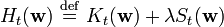
where optimization of S maximizes smoothness and  is known as a regularization parameter.
Interpolation[edit]
RBF networks can be used to interpolate a function  when the values of that function are known on finite number of points:
  . Taking the known points
  to be the centers of the radial basis functions and evaluating the values of the basis functions at the same points
 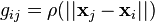 the weights can be solved from the equation
![\left[ \begin{matrix} g_{11} & g_{12} & \cdots & g_{1N} \\ g_{21} & g_{22} & \cdots & g_{2N} \\ \vdots & & \ddots & \vdots \\ g_{N1} & g_{N2} & \cdots & g_{NN} \end{matrix}\right] \left[ \begin{matrix} w_1 \\ w_2 \\ \vdots \\ w_N \end{matrix} \right] = \left[ \begin{matrix} b_1 \\ b_2 \\ \vdots \\ b_N \end{matrix} \right]](http://upload.wikimedia.org/math/6/a/3/6a329d7de56c97a7866e5cf0e650ba65.png)
It can be shown that the interpolation matrix in the above equation is non-singular, if the points are distinct, and thus the weights  can be solved by simple linear algebra:

Function approximation[edit]
If the purpose is not to perform strict interpolation but instead more general function approximation or classification the optimization is somewhat more complex because there is no obvious choice for the centers. The training is typically done in two phases first fixing the width and centers and then the weights. This can be justified by considering the different nature of the non-linear hidden neurons versus the linear output neuron.
Training the basis function centers[edit]
Basis function centers can be randomly sampled among the input instances or obtained by Orthogonal Least Square Learning Algorithm or found by clustering the samples and choosing the cluster means as the centers.
The RBF widths are usually all fixed to same value which is proportional to the maximum distance between the chosen centers.
Pseudoinverse solution for the linear weights[edit]
After the centers  have been fixed, the weights that minimize the error at the output are computed with a linearpseudoinverse solution:
 ,
,
where the entries of G are the values of the radial basis functions evaluated at the points  :
:  .
.
The existence of this linear solution means that unlike multi-layer perceptron (MLP) networks, RBF networks have a unique local minimum (when the centers are fixed).
Gradient descent training of the linear weights[edit]
Another possible training algorithm is gradient descent. In gradient descent training, the weights are adjusted at each time step by moving them in a direction opposite from the gradient of the objective function (thus allowing the minimum of the objective function to be found),
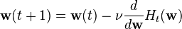
where  is a "learning parameter."
For the case of training the linear weights, , the algorithm becomes
![a_i (t+1) = a_i(t) + \nu \big [ y(t) - \varphi \big ( \mathbf{x}(t), \mathbf{w} \big ) \big ] \rho \big ( \left \Vert \mathbf{x}(t) - \mathbf{c}_i \right \Vert \big )](http://upload.wikimedia.org/math/6/b/2/6b2cd5d4c23386e2012ebcbaa424a4ed.png)
in the unnormalized case and
![a_i (t+1) = a_i(t) + \nu \big [ y(t) - \varphi \big ( \mathbf{x}(t), \mathbf{w} \big ) \big ] u \big ( \left \Vert \mathbf{x}(t) - \mathbf{c}_i \right \Vert \big )](http://upload.wikimedia.org/math/4/1/9/419021ac38cfb4f2f31bee6bb7ef9e0e.png)
in the normalized case.
For local-linear-architectures gradient-descent training is
![e_{ij} (t+1) = e_{ij}(t) + \nu \big [ y(t) - \varphi \big ( \mathbf{x}(t), \mathbf{w} \big ) \big ] v_{ij} \big ( \mathbf{x}(t) - \mathbf{c}_i \big )](http://upload.wikimedia.org/math/9/8/d/98d9700ab2fb374c88d7984697a8c4ad.png)
Projection operator training of the linear weights[edit]
For the case of training the linear weights, and  , the algorithm becomes
![a_i (t+1) = a_i(t) + \nu \big [ y(t) - \varphi \big ( \mathbf{x}(t), \mathbf{w} \big ) \big ] \frac {\rho \big ( \left \Vert \mathbf{x}(t) - \mathbf{c}_i \right \Vert \big )} {\sum_{i=1}^N \rho^2 \big ( \left \Vert \mathbf{x}(t) - \mathbf{c}_i \right \Vert \big )}](http://upload.wikimedia.org/math/9/5/e/95e0bdc7fb433ad19f80848c8c7080d7.png)
in the unnormalized case and
![a_i (t+1) = a_i(t) + \nu \big [ y(t) - \varphi \big ( \mathbf{x}(t), \mathbf{w} \big ) \big ] \frac {u \big ( \left \Vert \mathbf{x}(t) - \mathbf{c}_i \right \Vert \big )} {\sum_{i=1}^N u^2 \big ( \left \Vert \mathbf{x}(t) - \mathbf{c}_i \right \Vert \big )}](http://upload.wikimedia.org/math/3/7/c/37c01fc975b58cfde14effc94c4911ee.png)
in the normalized case and
![e_{ij} (t+1) = e_{ij}(t) + \nu \big [ y(t) - \varphi \big ( \mathbf{x}(t), \mathbf{w} \big ) \big ] \frac { v_{ij} \big ( \mathbf{x}(t) - \mathbf{c}_i \big ) } {\sum_{i=1}^N \sum_{j=1}^n v_{ij}^2 \big ( \mathbf{x}(t) - \mathbf{c}_i \big ) }](http://upload.wikimedia.org/math/9/9/9/99991b65a1bf7eb30e102b16ec292483.png)
in the local-linear case.
For one basis function, projection operator training reduces to Newton's method.

Figure 6: Logistic map time series. Repeated iteration of the logistic map generates a chaotic time series. The values lie between zero and one. Displayed here are the 100 training points used to train the examples in this section. The weights c are the first five points from this time series.
Examples[edit]
Logistic map[edit]
The basic properties of radial basis functions can be illustrated with a simple mathematical map, the logistic map, which maps the unit interval onto itself. It can be used to generate a convenient prototype data stream. The logistic map can be used to explore function approximation, time series prediction, and control theory. The map originated from the field of population dynamicsand became the prototype for chaotic time series. The map, in the fully chaotic regime, is given by
![x(t+1)\ \stackrel{\mathrm{def}}{=}\ f\left [ x(t)\right ] = 4 x(t) \left [ 1-x(t) \right ]](http://upload.wikimedia.org/math/c/b/2/cb29092162f637c2924e700b404f3104.png)
where t is a time index. The value of x at time t+1 is a parabolic function of x at time t. This equation represents the underlying geometry of the chaotic time series generated by the logistic map.
Generation of the time series from this equation is the forward problem. The examples here illustrate the inverse problem; identification of the underlying dynamics, or fundamental equation, of the logistic map from exemplars of the time series. The goal is to find an estimate
![x(t+1) = f \left [ x(t) \right ] \approx \varphi(t) = \varphi \left [ x(t)\right ]](http://upload.wikimedia.org/math/8/f/2/8f2f35ff674dc2314fcfa7be1cc0416b.png)
for f.
Function approximation[edit]
Unnormalized radial basis functions[edit]
The architecture is
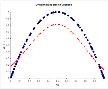
Figure 7: Unnormalized basis functions. The Logistic map (blue) and the approximation to the logistic map (red) after one pass through the training set.

where
![\rho \big ( \left \Vert \mathbf{x} - \mathbf{c}_i \right \Vert \big ) = \exp \left[ -\beta \left \Vert \mathbf{x} - \mathbf{c}_i \right \Vert ^2 \right] = \exp \left[ -\beta \left ( x(t) - c_i \right ) ^2 \right]](http://upload.wikimedia.org/math/0/5/3/0530388cea007f90c927565f114a8e0e.png) .
.
Since the input is a scalar rather than a vector, the input dimension is one. We choose the number of basis functions as N=5 and the size of the training set to be 100 exemplars generated by the chaotic time series. The weight  is taken to be a constant equal to 5. The weights are five exemplars from the time series. The weights are trained with projection operator training:
![a_i (t+1) = a_i(t) + \nu \big [ x(t+1) - \varphi \big ( \mathbf{x}(t), \mathbf{w} \big ) \big ] \frac {\rho \big ( \left \Vert \mathbf{x}(t) - \mathbf{c}_i \right \Vert \big )} {\sum_{i=1}^N \rho^2 \big ( \left \Vert \mathbf{x}(t) - \mathbf{c}_i \right \Vert \big )}](http://upload.wikimedia.org/math/4/0/7/4071758b40c6f5cfcefec99d7e18556b.png)
where the learning rate is taken to be 0.3. The training is performed with one pass through the 100 training points. Therms error is 0.15.
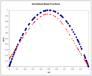
Figure 8: Normalized basis functions. The Logistic map (blue) and the approximation to the logistic map (red) after one pass through the training set. Note the improvement over the unnormalized case.
Normalized radial basis functions[edit]
The normalized RBF architecture is
where
 .
.
Again:
- .
Again, we choose the number of basis functions as five and the size of the training set to be 100 exemplars generated by the chaotic time series. The weight is taken to be a constant equal to 6. The weights are five exemplars from the time series. The weights are trained with projection operator training:
![a_i (t+1) = a_i(t) + \nu \big [ x(t+1) - \varphi \big ( \mathbf{x}(t), \mathbf{w} \big ) \big ] \frac {u \big ( \left \Vert \mathbf{x}(t) - \mathbf{c}_i \right \Vert \big )} {\sum_{i=1}^N u^2 \big ( \left \Vert \mathbf{x}(t) - \mathbf{c}_i \right \Vert \big )}](http://upload.wikimedia.org/math/7/c/d/7cdea8361f22e2e8e19b8e505ea39072.png)
where the learning rate is again taken to be 0.3. The training is performed with one pass through the 100 training points. The rms error on a test set of 100 exemplars is 0.084, smaller than the unnormalized error. Normalization yields accuracy improvement. Typically accuracy with normalized basis functions increases even more over unnormalized functions as input dimensionality increases.

Figure 9: Normalized basis functions. The Logistic map (blue) and the approximation to the logistic map (red) as a function of time. Note that the approximation is good for only a few time steps. This is a general characteristic of chaotic time series.
Time series prediction[edit]
Once the underlying geometry of the time series is estimated as in the previous examples, a prediction for the time series can be made by iteration:

![{x}(t+1) \approx \varphi(t)=\varphi [\varphi(t-1)]](http://upload.wikimedia.org/math/e/f/2/ef230570b4039f8a50961183a1885028.png) .
.
A comparison of the actual and estimated time series is displayed in the figure. The estimated times series starts out at time zero with an exact knowledge of x(0). It then uses the estimate of the dynamics to update the time series estimate for several time steps.
Note that the estimate is accurate for only a few time steps. This is a general characteristic of chaotic time series. This is a property of the sensitive dependence on initial conditions common to chaotic time series. A small initial error is amplified with time. A measure of the divergence of time series with nearly identical initial conditions is known as the Lyapunov exponent.
Control of a chaotic time series[edit]

Figure 10: Control of the logistic map. The system is allowed to evolve naturally for 49 time steps. At time 50 control is turned on. The desired trajectory for the time series is red. The system under control learns the underlying dynamics and drives the time series to the desired output. The architecture is the same as for the time series prediction example.
We assume the output of the logistic map can be manipulated through a control parameter ![c[ x(t),t]](http://upload.wikimedia.org/math/0/5/b/05bbd3576c59d2d858c7969d9bd15856.png) such that
such that
![{x}^{ }_{ }(t+1) = 4 x(t) [1-x(t)] +c[x(t),t]](http://upload.wikimedia.org/math/9/4/d/94deaf803d53e210470976bf835db56f.png) .
.
The goal is to choose the control parameter in such a way as to drive the time series to a desired output  . This can be done if we choose the control paramer to be
![c^{ }_{ }[x(t),t] \ \stackrel{\mathrm{def}}{=}\ -\varphi [x(t)] + d(t+1)](http://upload.wikimedia.org/math/9/d/7/9d7b2a1622bbda0acc9e95b7ceb8ec83.png)
where
![y[x(t)] \approx f[x(t)] = x(t+1)- c[x(t),t]](http://upload.wikimedia.org/math/c/9/a/c9ac6f37caa241d8fd033d380276ebaf.png)
is an approximation to the underlying natural dynamics of the system.
The learning algorithm is given by
where
![\varepsilon \ \stackrel{\mathrm{def}}{=}\ f[x(t)] - \varphi [x(t)] = x(t+1)- c[x(t),t] - \varphi [x(t)] = x(t+1) - d(t+1)](http://upload.wikimedia.org/math/6/b/2/6b285bb113b9acd3d55e2f7dd4ba93b4.png) .
.
See also[edit]
References[edit]
- J. Moody and C. J. Darken, "Fast learning in networks of locally tuned processing units," Neural Computation, 1, 281-294 (1989). Also see Radial basis function networks according to Moody and Darken
- T. Poggio and F. Girosi, "Networks for approximation and learning," Proc. IEEE 78(9), 1484-1487 (1990).
- Roger D. Jones, Y. C. Lee, C. W. Barnes, G. W. Flake, K. Lee, P. S. Lewis, and S. Qian, ?Function approximation and time series prediction with neural networks,? Proceedings of the International Joint Conference on Neural Networks, June 17-21, p. I-649 (1990).
- Martin D. Buhmann (2003). Radial Basis Functions: Theory and Implementations. Cambridge University. ISBN 0-521-63338-9.
- Yee, Paul V. and Haykin, Simon (2001). Regularized Radial Basis Function Networks: Theory and Applications. John Wiley. ISBN 0-471-35349-3.
- John R. Davies, Stephen V. Coggeshall, Roger D. Jones, and Daniel Schutzer, "Intelligent Security Systems," inFreedman, Roy S., Flein, Robert A., and Lederman, Jess, Editors (1995). Artificial Intelligence in the Capital Markets. Chicago: Irwin. ISBN 1-55738-811-3.
- Simon Haykin (1999). Neural Networks: A Comprehensive Foundation (2nd edition ed.). Upper Saddle River, NJ: Prentice Hall. ISBN 0-13-908385-5.
- S. Chen, C. F. N. Cowan, and P. M. Grant, "Orthogonal Least Squares Learning Algorithm for Radial Basis Function Networks", IEEE Transactions on Neural Networks, Vol 2, No 2 (Mar) 1991.