In statistics, an expectation–maximization (EM) algorithm is an iterative method for finding maximum likelihood ormaximum a posteriori (MAP) estimates of parameters in statistical models, where the model depends on unobservedlatent variables. The EM iteration alternates between performing an expectation (E) step, which creates a function for the expectation of the log-likelihood evaluated using the current estimate for the parameters, and a maximization (M) step, which computes parameters maximizing the expected log-likelihood found on the E step. These parameter-estimates are then used to determine the distribution of the latent variables in the next E step.

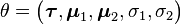
EM clustering of
Old Faithful eruption data. The random initial model (which due to the different scales of the axes appears to be two very flat and wide spheres) is fit to the observed data. In the first iterations, the model changes substantially, but then converges to the two modes of the
geyser. Visualized using
ELKI.
History[edit]
The EM algorithm was explained and given its name in a classic 1977 paper by Arthur Dempster, Nan Laird, and Donald Rubin.[1] They pointed out that the method had been "proposed many times in special circumstances" by earlier authors. In particular, a very detailed treatment of the EM method for exponential families was published by Rolf Sundberg in his thesis and several papers[2][3][4] following his collaboration with Per Martin-Löf and Anders Martin-Löf.[5][6][7][8][9][10][11] The Dempster-Laird-Rubin paper in 1977 generalized the method and sketched a convergence analysis for a wider class of problems. Regardless of earlier inventions, the innovative Dempster-Laird-Rubin paper in the Journal of the Royal Statistical Society received an enthusiastic discussion at the Royal Statistical Society meeting with Sundberg calling the paper "brilliant". The Dempster-Laird-Rubin paper established the EM method as an important tool of statistical analysis.
The convergence analysis of the Dempster-Laird-Rubin paper was flawed and a correct convergence analysis was published by C. F. Jeff Wu in 1983. Wu's proof established the EM method's convergence outside of the exponential family, as claimed by Dempster-Laird-Rubin.[12]
Introduction[edit]
The EM algorithm is used to find the maximum likelihood parameters of a statistical model in cases where the equations cannot be solved directly. Typically these models involve latent variables in addition to unknown parameters and known data observations. That is, either there are missing values among the data, or the model can be formulated more simply by assuming the existence of additional unobserved data points. (For example, a mixture model can be described more simply by assuming that each observed data point has a corresponding unobserved data point, or latent variable, specifying the mixture component that each data point belongs to.)
Finding a maximum likelihood solution requires taking the derivatives of the likelihood function with respect to all the unknown values — viz. the parameters and the latent variables — and simultaneously solving the resulting equations. In statistical models with latent variables, this usually is not possible. Instead, the result is typically a set of interlocking equations in which the solution to the parameters requires the values of the latent variables and vice-versa, but substituting one set of equations into the other produces an unsolvable equation.
The EM algorithm proceeds from the observation that the following is a way to solve these two sets of equations numerically. One can simply pick arbitrary values for one of the two sets of unknowns, use them to estimate the second set, then use these new values to find a better estimate of the first set, and then keep alternating between the two until the resulting values both converge to fixed points. It's not obvious that this will work at all, but in fact it can be proven that in this particular context it does, and that the derivative of the likelihood is (arbitrarily close to) zero at that point, which in turn means that the point is either a maximum or a saddle point.[citation needed] In general there may be multiple maxima, and no guarantee that the global maximum will be found. Some likelihoods also have singularities in them, i.e. nonsensical maxima. For example, one of the "solutions" that may be found by EM in a mixture model involves setting one of the components to have zero variance and the mean parameter for the same component to be equal to one of the data points.
Description[edit]
Given a statistical model consisting of a set  of observed data, a set of unobserved latent data or missing values
  , and a vector of unknown parameters
  , along with a likelihood function
  , the maximum likelihood estimate (MLE) of the unknown parameters is determined by the marginal likelihood of the observed data

However, this quantity is often intractable (e.g. if is a sequence of events, so that the number of values grows exponentially with the sequence length, making the exact calculation of the sum extremely difficult).
The EM algorithm seeks to find the MLE of the marginal likelihood by iteratively applying the following two steps:
- Expectation step (E step): Calculate the expected value of the log likelihood function, with respect to the conditional distribution of given under the current estimate of the parameters
 :
: ![Q(\boldsymbol\theta|\boldsymbol\theta^{(t)}) = \operatorname{E}_{\mathbf{Z}|\mathbf{X},\boldsymbol\theta^{(t)}}\left[ \log L (\boldsymbol\theta;\mathbf{X},\mathbf{Z}) \right] \,](http://upload.wikimedia.org/math/c/6/8/c685c42d963edd857fb2103a437b81c8.png)
- Maximization step (M step): Find the parameter that maximizes this quantity:
Note that in typical models to which EM is applied:
- The observed data points may be discrete (taking values in a finite or countably infinite set) or continuous(taking values in an uncountably infinite set). There may in fact be a vector of observations associated with each data point.
- The missing values (aka latent variables) are discrete, drawn from a fixed number of values, and there is one latent variable per observed data point.
- The parameters are continuous, and are of two kinds: Parameters that are associated with all data points, and parameters associated with a particular value of a latent variable (i.e. associated with all data points whose corresponding latent variable has a particular value).
However, it is possible to apply EM to other sorts of models.
The motivation is as follows. If we know the value of the parameters , we can usually find the value of the latent variables by maximizing the log-likelihood over all possible values of , either simply by iterating over or through an algorithm such as the Viterbi algorithm for hidden Markov models. Conversely, if we know the value of the latent variables , we can find an estimate of the parameters fairly easily, typically by simply grouping the observed data points according to the value of the associated latent variable and averaging the values, or some function of the values, of the points in each group. This suggests an iterative algorithm, in the case where both and are unknown:
- First, initialize the parameters to some random values.
- Compute the best value for given these parameter values.
- Then, use the just-computed values of to compute a better estimate for the parameters . Parameters associated with a particular value of will use only those data points whose associated latent variable has that value.
- Iterate steps 2 and 3 until convergence.
The algorithm as just described monotonically approaches a local minimum of the cost function, and is commonly calledhard EM. The k-means algorithm is an example of this class of algorithms.
However, we can do somewhat better by, rather than making a hard choice for given the current parameter values and averaging only over the set of data points associated with a particular value of , instead determining the probability of each possible value of for each data point, and then using the probabilities associated with a particular value of to compute a weighted average over the entire set of data points. The resulting algorithm is commonly called soft EM, and is the type of algorithm normally associated with EM. The counts used to compute these weighted averages are called soft counts (as opposed to the hard counts used in a hard-EM-type algorithm such as k-means). The probabilities computed for are posterior probabilities and are what is computed in the E step. The soft counts used to compute new parameter values are what is computed in the M step.
Properties[edit]
Speaking of an expectation (E) step is a bit of a misnomer. What is calculated in the first step are the fixed, data-dependent parameters of the function Q. Once the parameters of Q are known, it is fully determined and is maximized in the second (M) step of an EM algorithm.
Although an EM iteration does increase the observed data (i.e. marginal) likelihood function there is no guarantee that the sequence converges to a maximum likelihood estimator. For multimodal distributions, this means that an EM algorithm may converge to a local maximum of the observed data likelihood function, depending on starting values. There are a variety of heuristic or metaheuristic approaches for escaping a local maximum such as random restart (starting with several different random initial estimates θ(t)), or applying simulated annealing methods.
EM is particularly useful when the likelihood is an exponential family: the E step becomes the sum of expectations ofsufficient statistics, and the M step involves maximizing a linear function. In such a case, it is usually possible to deriveclosed form updates for each step, using the Sundberg formula (published by Rolf Sundberg using unpublished results ofPer Martin-Löf and Anders Martin-Löf).[3][4][7][8][9][10][11]
The EM method was modified to compute maximum a posteriori (MAP) estimates for Bayesian inference in the original paper by Dempster, Laird, and Rubin.
There are other methods for finding maximum likelihood estimates, such as gradient descent, conjugate gradient or variations of the Gauss–Newton method. Unlike EM, such methods typically require the evaluation of first and/or second derivatives of the likelihood function.
Proof of correctness[edit]
Expectation-maximization works to improve  rather than directly improving
  . Here we show that improvements to the former imply improvements to the latter.[13]
For any with non-zero probability  , we can write
-

We take the expectation over values of by multiplying both sides by  and summing (or integrating) over . The left-hand side is the expectation of a constant, so we get:
-

where  is defined by the negated sum it is replacing. This last equation holds for any value of including
  ,
,
-

and subtracting this last equation from the previous equation gives
-

However, Gibbs' inequality tells us that  , so we can conclude that
-

In words, choosing to improve beyond  will improve beyond
  at least as much.
Alternative description[edit]
Under some circumstances, it is convenient to view the EM algorithm as two alternating maximization steps.[14][15]Consider the function:
![F(q,\theta) = \operatorname{E}_q [ \log L (\theta ; x,Z) ] + H(q) = -D_{\mathrm{KL}}\big(q \big\| p_{Z|X}(\cdot|x;\theta ) \big) + \log L(\theta;x)](http://upload.wikimedia.org/math/c/a/4/ca41e0768b6a2bea24dd49b93685828d.png)
where q is an arbitrary probability distribution over the unobserved data z, pZ|X(· |x;θ) is the conditional distribution of the unobserved data given the observed data x, H is the entropy and DKL is the Kullback–Leibler divergence.
Then the steps in the EM algorithm may be viewed as:
- Expectation step: Choose q to maximize F:
- Maximization step: Choose θ to maximize F:
Applications[edit]
EM is frequently used for data clustering in machine learning and computer vision. In natural language processing, two prominent instances of the algorithm are the Baum-Welch algorithm (also known as forward-backward) and the inside-outside algorithm for unsupervised induction of probabilistic context-free grammars.
In psychometrics, EM is almost indispensable for estimating item parameters and latent abilities of item response theorymodels.
With the ability to deal with missing data and observe unidentified variables, EM is becoming a useful tool to price and manage risk of a portfolio.
The EM algorithm (and its faster variant Ordered subset expectation maximization) is also widely used in medical imagereconstruction, especially in positron emission tomography and single photon emission computed tomography. See below for other faster variants of EM.
Filtering and Smoothing EM Algorithms[edit]
A Kalman filter is typically used for on-line state estimation and a minimum-variance smoother may be employed for off-line or batch state estimation. However, these minimum-variance solutions require estimates of the state-space model parameters. EM algorithms can be used for solving joint state and parameter estimation problems.
Filtering and smoothing EM algorithms arise by repeating the following two-step procedure.
- E-Step
- Operate a Kalman filter or a minimum-variance smoother designed with current parameter estimates to obtain updated state estimates.
- M-Step
- Use the filtered or smoothed state estimates within maximum-likelihood calculations to obtain updated parameter estimates.
Suppose that a Kalman filter or minimum-variance smoother operates on noisy measurements of a single-input-single-output system. An updated measurement noise variance estimate can be obtained from the maximum likelihoodcalculation
where  are scalar output estimates calculated by a filter or a smoother from N scalar measurements
  . Similarly, for a first-order auto-regressive process, an updated process noise variance estimate can be calculated by

where and  are scalar state estimates calculated by a filter or a smoother. The updated model coefficient estimate is obtained via
 .
.
The convergence of parameter estimates such as those above are studied in[16] [17] .[18]
Variants[edit]
A number of methods have been proposed to accelerate the sometimes slow convergence of the EM algorithm, such as those utilising conjugate gradient and modified Newton–Raphson techniques.[19] Additionally EM can be utilised with constrained estimation techniques.
Expectation conditional maximization (ECM) replaces each M step with a sequence of conditional maximization (CM) steps in which each parameter θi is maximized individually, conditionally on the other parameters remaining fixed.[20]
This idea is further extended in generalized expectation maximization (GEM) algorithm, in which one only seeks an increase in the objective function F for both the E step and M step under the alternative description.[14]
It is also possible to consider the EM algorithm as a subclass of the MM (Majorize/Minimize or Minorize/Maximize, depending on context) algorithm,[21] and therefore use any machinery developed in the more general case.
α-EM algorithm[edit]
The Q-function used in the EM algorithm is based on the log likelihood. Therefore, it is regarded as the log-EM algorithm. The use of the log likelihood can be generalized to that of the α-log likelihood ratio. Then, the α-log likelihood ratio of the observed data can be exactly expressed as equality by using the Q-function of the α-log likelihood ratio and the α-divergence. Obtaining this Q-function is a generalized E step. Its maximization is a generalized M step. This pair is called the α-EM algorithm [22] which contains the log-EM algorithm as its subclass. Thus, the α-EM algorithm by Yasuo Matsuyama is an exact generalization of the log-EM algorithm. No computation of gradient or Hessian matrix is needed. The α-EM shows faster convergence than the log-EM algorithm by choosing an appropriate α. The α-EM algorithm leads to a faster version of the Hidden Markov model estimation algorithm α-HMM. [23]
Relation to variational Bayes methods[edit]
EM is a partially non-Bayesian, maximum likelihood method. Its final result gives a probability distribution over the latent variables (in the Bayesian style) together with a point estimate for θ (either a maximum likelihood estimate or a posterior mode). We may want a fully Bayesian version of this, giving a probability distribution over θ as well as the latent variables. In fact the Bayesian approach to inference is simply to treat θ as another latent variable. In this paradigm, the distinction between the E and M steps disappears. If we use the factorized Q approximation as described above (variational Bayes), we may iterate over each latent variable (now including θ) and optimize them one at a time. There are now k steps per iteration, where k is the number of latent variables. For graphical models this is easy to do as each variable's new Qdepends only on its Markov blanket, so local message passing can be used for efficient inference.
Geometric interpretation[edit]
In information geometry, the E step and the M step are interpreted as projections under dual affine connections, called the e-connection and the m-connection; the Kullback–Leibler divergence can also be understood in these terms.
Examples[edit]
Gaussian mixture[edit]
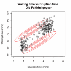
An animation demonstrating the EM algorithm fitting a two component Gaussian
mixture modelto the
Old Faithful dataset. The algorithm steps through from a random initialization to convergence.
Let x = (x1,x2,…,xn) be a sample of n independent observations from amixture of two multivariate normal distributions of dimension d, and let z=(z1,z2,…,zn) be the latent variables that determine the component from which the observation originates.[15]
 and
and 
where
 and
and 
The aim is to estimate the unknown parameters representing the "mixing" value between the Gaussians and the means and covariances of each:
where the likelihood function is:
where  is an indicator function and f is the probability density function of a multivariate normal. This may be rewritten inexponential family form:
![L(\theta;\mathbf{x},\mathbf{z}) = \exp \left\{ \sum_{i=1}^n \sum_{j=1}^2 \mathbb{I}(z_i=j) \big[ \log \tau_j -\tfrac{1}{2} \log |\sigma_j| -\tfrac{1}{2}(\mathbf{x}_i-\boldsymbol{\mu}_j)^\top\sigma_j^{-1} (\mathbf{x}_i-\boldsymbol{\mu}_j) -\tfrac{d}{2} \log(2\pi) \big] \right\}.](http://upload.wikimedia.org/math/6/f/a/6fa4da17289f44c456adfffef6bd162d.png)
To see the last equality, note that for each i all indicators  are equal to zero, except for one which is equal to one. The inner sum thus reduces to a single term.
Given our current estimate of the parameters θ(t), the conditional distribution of the Zi is determined by Bayes theorem to be the proportional height of the normal density weighted by τ:
 .
.
Thus, the E step results in the function:
![\begin{align}Q(\theta|\theta^{(t)}) &= \operatorname{E} [\log L(\theta;\mathbf{x},\mathbf{Z}) ] \\ &= \operatorname{E} [\log \prod_{i=1}^{n}L(\theta;\mathbf{x}_i,\mathbf{z}_i) ] \\ &= \operatorname{E} [\sum_{i=1}^n \log L(\theta;\mathbf{x}_i,\mathbf{z}_i) ] \\ &= \sum_{i=1}^n\operatorname{E} [\log L(\theta;\mathbf{x}_i,\mathbf{z}_i) ] \\ &= \sum_{i=1}^n \sum_{j=1}^2 T_{j,i}^{(t)} \big[ \log \tau_j -\tfrac{1}{2} \log |\sigma_j| -\tfrac{1}{2}(\mathbf{x}_i-\boldsymbol{\mu}_j)^\top\sigma_j^{-1} (\mathbf{x}_i-\boldsymbol{\mu}_j) -\tfrac{d}{2} \log(2\pi) \big] \end{align}](http://upload.wikimedia.org/math/9/5/3/953e2e10852fdced443d9256f068651f.png)
The quadratic form of Q(θ|θ(t)) means that determining the maximising values of θ is relatively straightforward. Note that τ, (μ1,Σ1) and (μ2,Σ2) may be all maximised independently of each other since they all appear in separate linear terms.
To begin, consider τ, which has the constraint τ1 + τ2=1:
![\begin{align}\boldsymbol{\tau}^{(t+1)} &= \underset{\boldsymbol{\tau}} {\operatorname{arg\,max}}\ Q(\theta | \theta^{(t)} ) \\ &= \underset{\boldsymbol{\tau}} {\operatorname{arg\,max}} \ \left\{ \left[ \sum_{i=1}^n T_{1,i}^{(t)} \right] \log \tau_1 + \left[ \sum_{i=1}^n T_{2,i}^{(t)} \right] \log \tau_2 \right\} \end{align}](http://upload.wikimedia.org/math/0/1/8/01848174797cfac4ae3385a8c168718f.png)
This has the same form as the MLE for the binomial distribution, so:

For the next estimates of (μ1,σ1):
This has the same form as a weighted MLE for a normal distribution, so
 and
and 
and, by symmetry:
 and
and  .
.
Termination[edit]
Break the iteration if  and
and  are close enough (below some preset threshold).
Generalization[edit]
The algorithm illustrated above can be generalized for mixture of multiple (more than two) multivariate normal distributions.
Truncated and censored regression[edit]
The EM algorithm has been implemented in the case where there is an underlying linear regression model explaining the variation of some quantity, but where the values actually observed are censored or truncated versions of those represented in the model.[24] Special cases of this model include censored or truncated observations from a single normal distribution.[24]
Further reading[edit]
- Robert Hogg, Joseph McKean and Allen Craig. Introduction to Mathematical Statistics. pp. 359–364. Upper Saddle River, NJ: Pearson Prentice Hall, 2005.
- The on-line textbook: Information Theory, Inference, and Learning Algorithms, by David J.C. MacKay includes simple examples of the EM algorithm such as clustering using the soft k-means algorithm, and emphasizes the variational view of the EM algorithm, as described in Chapter 33.7 of version 7.2 (fourth edition).
- Theory and Use of the EM Method by M. R. Gupta and Y. Chen is a well-written short book on EM, including detailed derivation of EM for GMMs, HMMs, and Dirichlet.
- Bilmes, Jeff. A Gentle Tutorial of the EM Algorithm and its Application to Parameter Estimation for Gaussian Mixture and Hidden Markov Models. CiteSeerX: 10.1.1.28.613, includes a simplified derivation of the EM equations for Gaussian Mixtures and Gaussian Mixture Hidden Markov Models.
- Variational Algorithms for Approximate Bayesian Inference, by M. J. Beal includes comparisons of EM to Variational Bayesian EM and derivations of several models including Variational Bayesian HMMs (chapters).
- Dellaert, Frank. The Expectation Maximization Algorithm. CiteSeerX: 10.1.1.9.9735, gives an easier explanation of EM algorithm in terms of lowerbound maximization.
- The Expectation Maximization Algorithm: A short tutorial, A self-contained derivation of the EM Algorithm by Sean Borman.
- The EM Algorithm, by Xiaojin Zhu.
- EM algorithm and variants: an informal tutorial by Alexis Roche. A concise and very clear description of EM and many interesting variants.
- Bishop, Christopher M. (2006). Pattern Recognition and Machine Learning. Springer. ISBN 0-387-31073-8.
- Einicke, G.A. (2012). Smoothing, Filtering and Prediction: Estimating the Past, Present and Future. Rijeka, Croatia: Intech. ISBN 978-953-307-752-9.
References[edit]
- Jump up^ Dempster, A.P.; Laird, N.M.; Rubin, D.B. (1977). "Maximum Likelihood from Incomplete Data via the EM Algorithm".Journal of the Royal Statistical Society, Series B 39 (1): 1–38. JSTOR 2984875. MR 0501537.
- Jump up^ Sundberg, Rolf (1974). "Maximum likelihood theory for incomplete data from an exponential family". Scandinavian Journal of Statistics 1 (2): 49–58. JSTOR 4615553. MR 381110.
- ^ Jump up to:a b Rolf Sundberg. 1971. Maximum likelihood theory and applications for distributions generated when observing a function of an exponential family variable. Dissertation, Institute for Mathematical Statistics, Stockholm University.
- ^ Jump up to:a b Sundberg, Rolf (1976). "An iterative method for solution of the likelihood equations for incomplete data from exponential families". Communications in Statistics – Simulation and Computation 5 (1): 55–64.doi:10.1080/03610917608812007. MR 443190.
- Jump up^ See the acknowledgement by Dempster, Laird and Rubin on pages 3, 5 and 11.
- Jump up^ G. Kulldorff. 1961. Contributions to the theory of estimation from grouped and partially grouped samples. Almqvist & Wiksell.
- ^ Jump up to:a b Anders Martin-Löf. 1963. "Utvärdering av livslängder i subnanosekundsområdet" ("Evaluation of sub-nanosecond lifetimes"). ("Sundberg formula")
- ^ Jump up to:a b Per Martin-Löf. 1966. Statistics from the point of view of statistical mechanics. Lecture notes, Mathematical Institute, Aarhus University. ("Sundberg formula" credited to Anders Martin-Löf).
- ^ Jump up to:a b Per Martin-Löf. 1970. Statistika Modeller (Statistical Models): Anteckningar från seminarier läsåret 1969–1970 (Notes from seminars in the academic year 1969-1970), with the assistance of Rolf Sundberg. Stockholm University. ("Sundberg formula")
- ^ Jump up to:a b Martin-Löf, P. The notion of redundancy and its use as a quantitative measure of the deviation between a statistical hypothesis and a set of observational data. With a discussion by F. Abildgård, A. P. Dempster, D. Basu, D. R. Cox, A. W. F. Edwards, D. A. Sprott, G. A. Barnard, O. Barndorff-Nielsen, J. D. Kalbfleisch and G. Rasch and a reply by the author.Proceedings of Conference on Foundational Questions in Statistical Inference (Aarhus, 1973), pp. 1–42. Memoirs, No. 1, Dept. Theoret. Statist., Inst. Math., Univ. Aarhus, Aarhus, 1974.
- ^ Jump up to:a b Martin-Löf, Per The notion of redundancy and its use as a quantitative measure of the discrepancy between a statistical hypothesis and a set of observational data. Scand. J. Statist. 1 (1974), no. 1, 3–18.
- Jump up^ Wu, C. F. Jeff (Mar. 1983). "On the Convergence Properties of the EM Algorithm". Annals of Statistics 11 (1): 95–103.doi:10.1214/aos/1176346060. JSTOR 2240463. MR 684867.
- Jump up^ Little, Roderick J.A.; Rubin, Donald B. (1987). Statistical Analysis with Missing Data. Wiley Series in Probability and Mathematical Statistics. New York: John Wiley & Sons. pp. 134–136. ISBN 0-471-80254-9.
- ^ Jump up to:a b Neal, Radford; Hinton, Geoffrey (1999). "A view of the EM algorithm that justifies incremental, sparse, and other variants". In Michael I. Jordan. Learning in Graphical Models (Cambridge, MA: MIT Press): 355–368. ISBN 0-262-60032-3. Retrieved 2009-03-22.
- ^ Jump up to:a b Hastie, Trevor; Tibshirani, Robert; Friedman, Jerome (2001). "8.5 The EM algorithm". The Elements of Statistical Learning. New York: Springer. pp. 236–243. ISBN 0-387-95284-5.
- Jump up^ Einicke, G.A.; Malos, J.T.; Reid, D.C.; Hainsworth, D.W. (January 2009). "Riccati Equation and EM Algorithm Convergence for Inertial Navigation Alignment". IEEE Trans. Signal Processing 57 (1): 370–375. doi:10.1109/TSP.2008.2007090
- Jump up^ Einicke, G.A.; Falco, G.; Malos, J.T. (May 2010). "EM Algorithm State Matrix Estimation for Navigation". IEEE Signal Processing Letters 17 (5): 437–440. Bibcode:2010ISPL...17..437E. doi:10.1109/LSP.2010.2043151
- Jump up^ Einicke, G.A.; Falco, G.; Dunn, M.T.; Reid, D.C. (May 2012). "Iterative Smoother-Based Variance Estimation". IEEE Signal Processing Letters 19 (5): 275–278. Bibcode:2012ISPL...19..275E. doi:10.1109/LSP.2012.2190278
- Jump up^ Jamshidian, Mortaza; Jennrich, Robert I. (1997). "Acceleration of the EM Algorithm by using Quasi-Newton Methods".Journal of the Royal Statistical Society, Series B 59 (2): 569–587. doi:10.1111/1467-9868.00083. MR 1452026.
- Jump up^ Meng, Xiao-Li; Rubin, Donald B. (1993). "Maximum likelihood estimation via the ECM algorithm: A general framework".Biometrika 80 (2): 267–278. doi:10.1093/biomet/80.2.267. MR 1243503.
- Jump up^ Hunter DR and Lange K (2004), A Tutorial on MM Algorithms, The American Statistician, 58: 30-37
- Jump up^ Matsuyama, Yasuo (2003). "The α-EM algorithm: Surrogate likelihood maximization using α-logarithmic information measures". IEEE Transactions on Information Theory 49 (3): 692–706. doi:10.1109/TIT.2002.808105.
- Jump up^ Matsuyama, Yasuo (2011). "Hidden Markov model estimation based on alpha-EM algorithm: Discrete and continuous alpha-HMMs". International Joint Conference on Neural Networks: 808–816.
- ^ Jump up to:a b Wolynetz, M.S. (1979). "Maximum likelihood estimation in a linear model from confined and censored normal data".Journal of the Royal Statistical Society, Series C 28 (2): 195–206.
External links[edit]