Details view: Data clustering

Machine learning andData mining

Problems
Classification Clustering Regression Anomaly detection Association rules Reinforcement learning Structured prediction Feature learning Online learning Semi-supervised learning Grammar induction
Supervised learning (classification,regression)
Decision trees k-NN Linear regression Naive Bayes Logistic regression SVM Neural networks
Clustering
Hierarchical k-means EM DBSCAN OPTICS Mean-shift
Anomaly detection
k-NN Local outlier factor
Theory
Bias-variance dilemma Computational learning theory Empirical risk minimization PAC learning VC theory
Computer science portal Statistics portal
v t e

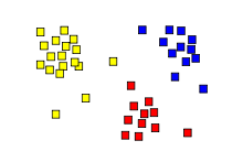
The result of a cluster analysis shown as the coloring of the squares into three clusters.

This section needs additional citations forverification. Please help improve this article byadding citations to reliable sources. Unsourced material may be challenged and removed. (May 2012)

Cluster analysis or clustering is the task of grouping a set of objects in such a way that objects in the same group (called a cluster) are more similar (in some sense or another) to each other than to those in other groups (clusters). It is a main task of exploratory data mining, and a common technique for statistical data analysis, used in many fields, including machine learning, pattern recognition, image analysis, information retrieval, andbioinformatics.

Cluster analysis itself is not one specific algorithm, but the general task to be solved. It can be achieved by various algorithms that differ significantly in their notion of what constitutes a cluster and how to efficiently find them. Popular notions of clusters include groups with small distances among the cluster members, dense areas of the data space, intervals or particular statistical distributions. Clustering can therefore be formulated as a multi-objective optimization problem. The appropriate clustering algorithm and parameter settings (including values such as the distance function to use, a density threshold or the number of expected clusters) depend on the individual data set and intended use of the results. Cluster analysis as such is not an automatic task, but an iterative process of knowledge discovery or interactive multi-objective optimization that involves trial and failure. It will often be necessary to modify data preprocessing and model parameters until the result achieves the desired properties.

Besides the term clustering, there are a number of terms with similar meanings, including automatic classification, numerical taxonomy, botryology(from Greek βότρυς "grape") and typological analysis. The subtle differences are often in the usage of the results: while in data mining, the resulting groups are the matter of interest, in automatic classification primarily their discriminative power is of interest. This often leads to misunderstandings between researchers coming from the fields of data mining and machine learning, since they use the same terms and often the same algorithms, but have different goals.

Cluster analysis was originated in anthropology by Driver and Kroeber in 1932 and introduced to psychology by Zubin in 1938 and Robert Tryon in 1939^[1]^[2]and famously used by Cattell beginning in 1943^[3] for trait theory classification in personality psychology.

Clusters and clusterings[edit]

According to Vladimir Estivill-Castro, the notion of a "cluster" cannot be precisely defined, which is one of the reasons why there are so many clustering algorithms.^[4] There is a common denominator: a group of data objects. However, different researchers employ different cluster models, and for each of these cluster models again different algorithms can be given. The notion of a cluster, as found by different algorithms, varies significantly in its properties. Understanding these "cluster models" is key to understanding the differences between the various algorithms. Typical cluster models include:

Connectivity models: for example hierarchical clustering builds models based on distance connectivity.
Centroid models: for example the k-means algorithm represents each cluster by a single mean vector.
Distribution models: clusters are modeled using statistical distributions, such as multivariate normal distributions used by the Expectation-maximization algorithm.
Density models: for example DBSCAN and OPTICS defines clusters as connected dense regions in the data space.
Subspace models: in Biclustering (also known as Co-clustering or two-mode-clustering), clusters are modeled with both cluster members and relevant attributes.
Group models: some algorithms do not provide a refined model for their results and just provide the grouping information.
Graph-based models: a clique, i.e., a subset of nodes in a graph such that every two nodes in the subset are connected by an edge can be considered as a prototypical form of cluster. Relaxations of the complete connectivity requirement (a fraction of the edges can be missing) are known as quasi-cliques.

A "clustering" is essentially a set of such clusters, usually containing all objects in the data set. Additionally, it may specify the relationship of the clusters to each other, for example a hierarchy of clusters embedded in each other. Clusterings can be roughly distinguished as:

hard clustering: each object belongs to a cluster or not
soft clustering (also: fuzzy clustering): each object belongs to each cluster to a certain degree (e.g. a likelihood of belonging to the cluster)

There are also finer distinctions possible, for example:

strict partitioning clustering: here each object belongs to exactly one cluster
strict partitioning clustering with outliers: objects can also belong to no cluster, and are considered outliers.
overlapping clustering (also: alternative clustering, multi-view clustering): while usually a hard clustering, objects may belong to more than one cluster.
hierarchical clustering: objects that belong to a child cluster also belong to the parent cluster
subspace clustering: while an overlapping clustering, within a uniquely defined subspace, clusters are not expected to overlap.

Clustering algorithms[edit]

Clustering algorithms can be categorized based on their cluster model, as listed above. The following overview will only list the most prominent examples of clustering algorithms, as there are possibly over 100 published clustering algorithms. Not all provide models for their clusters and can thus not easily be categorized. An overview of algorithms explained in Wikipedia can be found in the list of statistics algorithms.

There is no objectively "correct" clustering algorithm, but as it was noted, "clustering is in the eye of the beholder."^[4] The most appropriate clustering algorithm for a particular problem often needs to be chosen experimentally, unless there is a mathematical reason to prefer one cluster model over another. It should be noted that an algorithm that is designed for one kind of model has no chance on a data set that contains a radically different kind of model.^[4] For example, k-means cannot find non-convex clusters.^[4]

Connectivity based clustering (hierarchical clustering)[edit]

Main article: Hierarchical clustering

Connectivity based clustering, also known as hierarchical clustering, is based on the core idea of objects being more related to nearby objects than to objects farther away. These algorithms connect "objects" to form "clusters" based on their distance. A cluster can be described largely by the maximum distance needed to connect parts of the cluster. At different distances, different clusters will form, which can be represented using a dendrogram, which explains where the common name "hierarchical clustering" comes from: these algorithms do not provide a single partitioning of the data set, but instead provide an extensive hierarchy of clusters that merge with each other at certain distances. In a dendrogram, the y-axis marks the distance at which the clusters merge, while the objects are placed along the x-axis such that the clusters don't mix.

Connectivity based clustering is a whole family of methods that differ by the way distances are computed. Apart from the usual choice of distance functions, the user also needs to decide on the linkage criterion (since a cluster consists of multiple objects, there are multiple candidates to compute the distance to) to use. Popular choices are known as single-linkage clustering (the minimum of object distances), complete linkage clustering (the maximum of object distances) orUPGMA ("Unweighted Pair Group Method with Arithmetic Mean", also known as average linkage clustering). Furthermore, hierarchical clustering can be agglomerative (starting with single elements and aggregating them into clusters) or divisive (starting with the complete data set and dividing it into partitions).

These methods will not produce a unique partitioning of the data set, but a hierarchy from which the user still needs to choose appropriate clusters. They are not very robust towards outliers, which will either show up as additional clusters or even cause other clusters to merge (known as "chaining phenomenon", in particular with single-linkage clustering). In the general case, the complexity is $\mathcal{O}(n^3)$ , which makes them too slow for large data sets. For some special cases, optimal efficient methods (of complexity $\mathcal{O}(n^2)$ ) are known: SLINK^[5] for single-linkage and CLINK^[6] for complete-linkage clustering. In the data mining community these methods are recognized as a theoretical foundation of cluster analysis, but often considered obsolete. They did however provide inspiration for many later methods such as density based clustering.

Linkage clustering examples
Single-linkage on Gaussian data. At 35 clusters, the biggest cluster starts fragmenting into smaller parts, while before it was still connected to the second largest due to the single-link effect.
Single-linkage on density-based clusters. 20 clusters extracted, most of which contain single elements, since linkage clustering does not have a notion of "noise".

Centroid-based clustering[edit]

Main article: k-means clustering

In centroid-based clustering, clusters are represented by a central vector, which may not necessarily be a member of the data set. When the number of clusters is fixed to k, k-means clustering gives a formal definition as an optimization problem: find the $k$ cluster centers and assign the objects to the nearest cluster center, such that the squared distances from the cluster are minimized.

The optimization problem itself is known to be NP-hard, and thus the common approach is to search only for approximate solutions. A particularly well known approximative method is Lloyd's algorithm,^[7] often actually referred to as "k-means algorithm". It does however only find a local optimum, and is commonly run multiple times with different random initializations. Variations of k-means often include such optimizations as choosing the best of multiple runs, but also restricting the centroids to members of the data set (k-medoids), choosing medians (k-medians clustering), choosing the initial centers less randomly (K-means++) or allowing a fuzzy cluster assignment (Fuzzy c-means).

Most k-means-type algorithms require the number of clusters - $k$ - to be specified in advance, which is considered to be one of the biggest drawbacks of these algorithms. Furthermore, the algorithms prefer clusters of approximately similar size, as they will always assign an object to the nearest centroid. This often leads to incorrectly cut borders in between of clusters (which is not surprising, as the algorithm optimized cluster centers, not cluster borders).

K-means has a number of interesting theoretical properties. On the one hand, it partitions the data space into a structure known as a Voronoi diagram. On the other hand, it is conceptually close to nearest neighbor classification, and as such is popular in machine learning. Third, it can be seen as a variation of model based classification, and Lloyd's algorithm as a variation of the Expectation-maximization algorithm for this model discussed below.

k-Means clustering examples
K-means separates data into Voronoi-cells, which assumes equal-sized clusters (not adequate here)
K-means cannot represent density-based clusters

Distribution-based clustering[edit]

The clustering model most closely related to statistics is based on distribution models. Clusters can then easily be defined as objects belonging most likely to the same distribution. A nice property of this approach is that this closely resembles the way artificial data sets are generated: by sampling random objects from a distribution.

While the theoretical foundation of these methods is excellent, they suffer from one key problem known as overfitting, unless constraints are put on the model complexity. A more complex model will usually always be able to explain the data better, which makes choosing the appropriate model complexity inherently difficult.

One prominent method is known as Gaussian mixture models (using the expectation-maximization algorithm). Here, the data set is usually modelled with a fixed (to avoid overfitting) number of Gaussian distributions that are initialized randomly and whose parameters are iteratively optimized to fit better to the data set. This will converge to a local optimum, so multiple runs may produce different results. In order to obtain a hard clustering, objects are often then assigned to the Gaussian distribution they most likely belong to; for soft clusterings, this is not necessary.

Distribution-based clustering is a semantically strong^{[clarification needed]} method, as it not only provides you with clusters, but also produces complex models for the clusters that can also capture correlation and dependence of attributes. However, using these algorithms puts an extra burden on the user: to choose appropriate data models to optimize, and for many real data sets, there may be no mathematical model available the algorithm is able to optimize (e.g. assuming Gaussian distributions is a rather strong assumption on the data).

Expectation-Maximization (EM) clustering examples
On Gaussian-distributed data, EM works well, since it uses Gaussians for modelling clusters
Density-based clusters cannot be modeled using Gaussian distributions

Density-based clustering[edit]

In density-based clustering,^[8] clusters are defined as areas of higher density than the remainder of the data set. Objects in these sparse areas - that are required to separate clusters - are usually considered to be noise and border points.

The most popular^[9] density based clustering method is DBSCAN.^[10] In contrast to many newer methods, it features a well-defined cluster model called "density-reachability". Similar to linkage based clustering, it is based on connecting points within certain distance thresholds. However, it only connects points that satisfy a density criterion, in the original variant defined as a minimum number of other objects within this radius. A cluster consists of all density-connected objects (which can form a cluster of an arbitrary shape, in contrast to many other methods) plus all objects that are within these objects' range. Another interesting property of DBSCAN is that its complexity is fairly low - it requires a linear number of range queries on the database - and that it will discover essentially the same results (it is deterministic for core and noise points, but not for border points) in each run, therefore there is no need to run it multiple times. OPTICS^[11] is a generalization of DBSCAN that removes the need to choose an appropriate value for the range parameter $\varepsilon$ , and produces a hierarchical result related to that of linkage clustering. DeLi-Clu,^[12] Density-Link-Clustering combines ideas from single-linkage clustering and OPTICS, eliminating the $\varepsilon$ parameter entirely and offering performance improvements over OPTICS by using an R-tree index.

The key drawback of DBSCAN and OPTICS is that they expect some kind of density drop to detect cluster borders. Moreover, they cannot detect intrinsic cluster structures which are prevalent in the majority of real life data. A variation of DBSCAN, EnDBSCAN,^[13] efficiently detects such kinds of structures. On data sets with, for example, overlapping Gaussian distributions - a common use case in artificial data - the cluster borders produced by these algorithms will often look arbitrary, because the cluster density decreases continuously. On a data set consisting of mixtures of Gaussians, these algorithms are nearly always outperformed by methods such as EM clustering that are able to precisely model this kind of data.

Density-based clustering examples
Density-based clustering with DBSCAN.
DBSCAN assumes clusters of similar density, and may have problems separating nearby clusters
OPTICS is a DBSCAN variant that handles different densities much better

Recent developments[edit]

In recent years considerable effort has been put into improving algorithm performance of the existing algorithms.^[14]^[15]Among them are CLARANS (Ng and Han, 1994),^[16] and BIRCH (Zhang et al., 1996).^[17] With the recent need to process larger and larger data sets (also known as big data), the willingness to trade semantic meaning of the generated clusters for performance has been increasing. This led to the development of pre-clustering methods such as canopy clustering, which can process huge data sets efficiently, but the resulting "clusters" are merely a rough pre-partitioning of the data set to then analyze the partitions with existing slower methods such as k-means clustering. Various other approaches to clustering have been tried such as seed based clustering.^[18]

For high-dimensional data, many of the existing methods fail due to the curse of dimensionality, which renders particular distance functions problematic in high-dimensional spaces. This led to new clustering algorithms for high-dimensional datathat focus on subspace clustering (where only some attributes are used, and cluster models include the relevant attributes for the cluster) and correlation clustering that also looks for arbitrary rotated ("correlated") subspace clusters that can be modeled by giving a correlation of their attributes. Examples for such clustering algorithms are CLIQUE^[19] andSUBCLU.^[20]

Ideas from density-based clustering methods (in particular the DBSCAN/OPTICS family of algorithms) have been adopted to subspace clustering (HiSC,^[21] hierarchical subspace clustering and DiSH^[22]) and correlation clustering (HiCO,^[23]hierarchical correlation clustering, 4C^[24] using "correlation connectivity" and ERiC^[25] exploring hierarchical density-based correlation clusters).

Several different clustering systems based on mutual information have been proposed. One is Marina Meilă's variation of information metric;^[26] another provides hierarchical clustering.^[27] Using genetic algorithms, a wide range of different fit-functions can be optimized, including mutual information.^[28] Also message passing algorithms, a recent development inComputer Science and Statistical Physics, has led to the creation of new types of clustering algorithms.^[29]

Evaluation of clustering results[edit]

Evaluation of clustering results sometimes is referred to as cluster validation.

There have been several suggestions for a measure of similarity between two clusterings. Such a measure can be used to compare how well different data clustering algorithms perform on a set of data. These measures are usually tied to the type of criterion being considered in assessing the quality of a clustering method.

Internal evaluation[edit]

When a clustering result is evaluated based on the data that was clustered itself, this is called internal evaluation. These methods usually assign the best score to the algorithm that produces clusters with high similarity within a cluster and low similarity between clusters. One drawback of using internal criteria in cluster evaluation is that high scores on an internal measure do not necessarily result in effective information retrieval applications.^[30] Additionally, this evaluation is biased towards algorithms that use the same cluster model. For example k-Means clustering naturally optimizes object distances, and a distance-based internal criterion will likely overrate the resulting clustering.

Therefore, the internal evaluation measures are best suited to get some insight into situations where one algorithm performs better than another, but this shall not imply that one algorithm produces more valid results than another.^[4]Validity as measured by such an index depends on the claim that this kind of structure exists in the data set. An algorithm designed for some kind of models has no chance if the data set contains a radically different set of models, or if the evaluation measures a radically different criterion.^[4] For example, k-means clustering can only find convex clusters, and many evaluation indexes assume convex clusters. On a data set with non-convex clusters neither the use of k-means, nor of an evaluation criterion that assumes convexity, is sound.

The following methods can be used to assess the quality of clustering algorithms based on internal criterion:

Linear Algebra Measure (Laura A Mather, 2000, JASIST 51:602-613)

One of the most common models in information retrieval (IR), the vector space model, represents a document set as a term-document matrix where each row corresponds to a term and each column corresponds to a document. Because of the use of matrices in IR, it is possible to apply linear algebra to this IR model. This paper describes an application of linear algebra to text clustering, namely, a metric for measuring cluster quality. The metric is based on the theory that cluster quality is proportional to the number of terms that are disjoint across the clusters. The metric compares the singular values of the term-document matrix to the singular values of the matrices for each of the clusters to determine the amount of overlap of the terms across clusters. Because the metric can be difficult to interpret, a standardization of the metric is defined, which specifies the number of standard deviations a clustering of a document set is from an average, random clustering of that document set. Empirical evidence shows that the standardized cluster metric correlates with clustered retrieval performance when comparing clustering algorithms or multiple parameters for the same clustering algorithm.

Davies–Bouldin index

The Davies–Bouldin index can be calculated by the following formula:

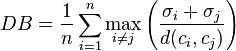
$DB = \frac {1} {n} \sum_{i=1}^{n} \max_{i\neq j}\left(\frac{\sigma_i + \sigma_j} {d(c_i,c_j)}\right)$

where n is the number of clusters, $c_x$ is the centroid of cluster $x$ , $\sigma_x$ is the average distance of all elements in cluster $x$ to centroid $c_x$ , and $d(c_i,c_j)$ is the distance between centroids $c_i$ and $c_j$ . Since algorithms that produce clusters with low intra-cluster distances (high intra-cluster similarity) and high inter-cluster distances (low inter-cluster similarity) will have a low Davies–Bouldin index, the clustering algorithm that produces a collection of clusters with the smallestDavies–Bouldin index is considered the best algorithm based on this criterion.

Dunn index (J. C. Dunn 1974)

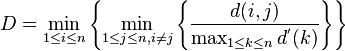
The Dunn index aims to identify dense and well-separated clusters. It is defined as the ratio between the minimal inter-cluster distance to maximal intra-cluster distance. For each cluster partition, the Dunn index can be calculated by the following formula:^[31]

$D = \min_{1\leq i \leq n}\left\{\min_{1\leq j \leq n,i\neq j}\left\{\frac {d(i,j)}{\max_{1\leq k \leq n}{d^{'}(k)}}\right\}\right\}$

where $d(i,j)$ represents the distance between clusters $i$ and $j$ , and $d^{'}(k)$ measures the intra-cluster distance of cluster $k$ . The inter-cluster distance $d(i,j)$ between two clusters may be any number of distance measures, such as the distance between the centroids of the clusters. Similarly, the intra-cluster distance $d^{'}(k)$ may be measured in a variety ways, such as the maximal distance between any pair of elements in cluster $k$ . Since internal criterion seek clusters with high intra-cluster similarity and low inter-cluster similarity, algorithms that produce clusters with high Dunn index are more desirable.

External evaluation[edit]

In external evaluation, clustering results are evaluated based on data that was not used for clustering, such as known class labels and external benchmarks. Such benchmarks consist of a set of pre-classified items, and these sets are often created by human (experts). Thus, the benchmark sets can be thought of as a gold standard for evaluation. These types of evaluation methods measure how close the clustering is to the predetermined benchmark classes. However, it has recently been discussed whether this is adequate for real data, or only on synthetic data sets with a factual ground truth, since classes can contain internal structure, the attributes present may not allow separation of clusters or the classes may contain anomalies.^[32] Additionally, from a knowledge discovery point of view, the reproduction of known knowledge may not necessarily be the intended result.^[32]

Some of the measures of quality of a cluster algorithm using external criterion include:

Rand measure (William M. Rand 1971)^[33]

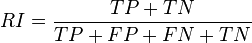
The Rand index computes how similar the clusters (returned by the clustering algorithm) are to the benchmark classifications. One can also view the Rand index as a measure of the percentage of correct decisions made by the algorithm. It can be computed using the following formula:

$RI = \frac {TP + TN} {TP + FP + FN + TN}$

where $TP$ is the number of true positives, $TN$ is the number of true negatives, $FP$ is the number of false positives, and $FN$ is the number of false negatives. One issue with the Rand index is that false positives and false negatives are equally weighted. This may be an undesirable characteristic for some clustering applications. The F-measure addresses this concern.

F-measure

The F-measure can be used to balance the contribution of false negatives by weighting recall through a parameter $\beta \geq 0$ . Let precision and recall be defined as follows:

$P = \frac {TP } {TP + FP }$

$R = \frac {TP } {TP + FN}$

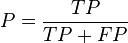
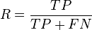
where $P$ is the precision rate and $R$ is the recall rate. We can calculate the F-measure by using the following formula:^[30]

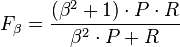
$F_{\beta} = \frac {(\beta^2 + 1)\cdot P \cdot R } {\beta^2 \cdot P + R}$

Notice that when $\beta=0$ , $F_{0}=P$ . In other words, recall has no impact on the F-measure when $\beta=0$ , and increasing $\beta$ allocates an increasing amount of weight to recall in the final F-measure.

Pair-counting F-Measure is the F-Measure applied to the set of object pairs, where objects are paired with each other when they are part of the same cluster. This measure is able to compare clusterings with different numbers of clusters.
Jaccard index

The Jaccard index is used to quantify the similarity between two datasets. The Jaccard index takes on a value between 0 and 1. An index of 1 means that the two dataset are identical, and an index of 0 indicates that the datasets have no common elements. The Jaccard index is defined by the following formula:

$J(A,B) = \frac {|A \cap B| } {|A \cup B|} = \frac{TP}{TP + FP + FN}$

This is simply the number of unique elements common to both sets divided by the total number of unique elements in both sets.

Fowlkes–Mallows index (E. B. Fowlkes & C. L. Mallows 1983)^[34]

The Fowlkes-Mallows index computes the similarity between the clusters returned by the clustering algorithm and the benchmark classifications. The higher the value of the Fowlkes-Mallows index the more similar the clusters and the benchmark classifications are. It can be computed using the following formula:

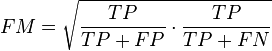
$FM = \sqrt{ \frac {TP}{TP+FP} \cdot \frac{TP}{TP+FN} }$

where $TP$ is the number of true positives, $FP$ is the number of false positives, and $FN$ is the number of false negatives. The $FM$ index is the geometric mean of the precision and recall $P$ and $R$ , while the F-measure is their harmonic mean.^[35] Moreover, precision and recall are also known as Wallace's indices $B^I$ and $B^{II}$ .^[36]

Confusion matrix

A confusion matrix can be used to quickly visualize the results of a classification (or clustering) algorithm. It shows how different a cluster is from the gold standard cluster.

The Mutual Information is an information theoretic measure of how much information is shared between a clustering and a ground-truth classification that can detect a non-linear similarity between two clusterings. Adjusted mutual information is the corrected-for-chance variant of this that has a reduced bias for varying cluster numbers.

Clustering Axioms[edit]

Given that there is a myriad of clustering algorithms and objectives, it is helpful to reason about clustering independently of any particular algorithm, objective function, or generative data model. This can be achieved by defining a clustering function as one that satisfies a set of properties. This is often termed as an Axiomatic System. Functions that satisfy the basic axioms are called clustering functions.^[37]

Formal Preliminaries[edit]

A partitioning function acts on a set $S$ of $n \ge 2$ points along with an integer $k > 0$ , and pairwise distances among the points in $S$ . The points are not assumed to belong to any specific larger set or space; the pairwise distances are the only data the partitioning function has about them.^{[citation needed]} We may label the points in $S$ using the numbers $\{1, 2, \ldots, n\}$ . The pairwise distances define a distance function $d: S \times S \rightarrow R$ which should have the properties of a semimetric: for any $i, j \in S$ , we must have $d(i, j) \ge 0, d(i, j) = d(j, i)$ , and $d(i, j) = 0$ if and only if $i = j$ . In other words, the distances must be nonnegative, symmetric, and two points have distance zero if only if they are the same point.

A partitioning function $F$ takes a distance function $d$ on $S \times S$ and an integer $k \ge 1$ and returns a $k$ -partition of $S$ , a collection of non-empty disjoint subsets of $S$ whose union is $S$ . The sets making up the k-partition are the clusters. Two clustering functions are equivalent if and only if they output the same partitioning on all values of $d$ and $k$ .

Axioms[edit]

Now in an effort to distinguish clustering functions from partitioning functions, we lay down some properties that one may like a clustering function to satisfy. Here is the first one. If $d$ is a distance function, then we define $\alpha \cdot d$ to be the same function with all distances multiplied by $\alpha$ .

Scale-Invariance.

For any distance function $d$ , number of clusters $k$ , and scalar $\alpha > 0$ , we have $F(d, k) = F(\alpha \cdot d, k)$

This property simply requires the function to be immune to stretching or shrinking the data points linearly. It effectively disallows clustering functions to be sensitive to changes in units of measurement - which is desirable. We would like clustering functions to not have any predefined hard-coded distance values in their decision process.

The next property ensures that the clustering function is “rich" in types of partitioning it could output. For a fixed $S$ and $k$ , Let Range( $F(\bullet , k)$ ) be the set of all possible outputs while varying $d$ .

$k$ -Richess.

For any number of clusters $k$ , Range( $F(\bullet, k)$ ) is equal to the set of all $k$ -partitions of $S$

In other words, if we are given a set of points such that all we know about the points are pairwise distances, then for any partitioning $\Gamma$ , there should exist a $d$ such that $F(d, k) = \Gamma$ . By varying distances amongst points, we should be able to obtain all possible $k$ -partitionings.

The next property is more subtle. We call a partitioning function “consistent" if it satisfies the following: when we shrink distances between points in the same cluster and expand distances between points in different clusters, we get the same result. Formally, we say that $d'$ is a $\Gamma$ -transformation of $d$ if (a) for all $i,j \in S$ belonging to the same cluster of $\Gamma$ , we have $d'(i,j) \le d(i,j)$ ; and (b) for all $i,j \in S$ belonging to different clusters of $\Gamma$ , we have $d'(i,j) \ge d(i,j)$ . In other words, $d'$ is a transformation of $d$ such that points inside the same cluster are brought closer together and points not inside the same cluster are moved further away from one another.

Consistency.

Fix $k$ . Let $d$ be a distance function, and $d'$ be a $F(d, k)$ -transformation of $d$ . Then $F(d, k) = F(d', k)$

In other words, suppose that we run the partitioning function $F$ on $d$ to get back a particular partitioning $\Gamma$ . Now, with respect to $\Gamma$ , if we shrink in-cluster distances or expand between-cluster distances and run $F$ again, we should still get back the same result - namely $\Gamma$ .

The partitioning function $F$ is forced to return a fixed number of clusters: $k$ . If this were not the case, then the above three properties could never be satisfied by any function.^[38] In many popular clustering algorithms such as $k$ -means, Single-Linkage, and spectral clustering, the number of clusters to be returned is determined beforehand – by the human user or other methods – and passed into the clustering function as a parameter.

Applications[edit]

Biology, computational biology and bioinformatics

Plant and animal ecology: cluster analysis is used to describe and to make spatial and temporal comparisons of communities (assemblages) of organisms in heterogeneous environments; it is also used in plant systematics to generate artificial phylogeniesor clusters of organisms (individuals) at the species, genus or higher level that share a number of attributes
Transcriptomics: clustering is used to build groups of genes with related expression patterns (also known as coexpressed genes). Often such groups contain functionally related proteins, such as enzymes for a specific pathway, or genes that are co-regulated. High throughput experiments using expressed sequence tags (ESTs) or DNA microarrays can be a powerful tool for genome annotation, a general aspect of genomics.
Sequence analysis: clustering is used to group homologous sequences into gene families. This is a very important concept in bioinformatics, and evolutionary biology in general. See evolution by gene duplication.
High-throughput genotyping platforms: clustering algorithms are used to automatically assign genotypes.
Human genetic clustering: The similarity of genetic data is used in clustering to infer population structures.

Medicine

Medical imaging: On PET scans, cluster analysis can be used to differentiate between different types of tissue and blood in a three dimensional image. In this application, actual position does not matter, but the voxel intensity is considered as avector, with a dimension for each image that was taken over time. This technique allows, for example, accurate measurement of the rate a radioactive tracer is delivered to the area of interest, without a separate sampling ofarterial blood, an intrusive technique that is most common today.
IMRT segmentation: Clustering can be used to divide a fluence map into distinct regions for conversion into deliverable fields in MLC-based Radiation Therapy.

Business and marketing

Market research: Cluster analysis is widely used in market research when working with multivariate data from surveys and test panels. Market researchers use cluster analysis to partition the general population of consumers into market segments and to better understand the relationships between different groups of consumers/potential customers, and for use in market segmentation, Product positioning, New product development and Selecting test markets.
Grouping of shopping items: Clustering can be used to group all the shopping items available on the web into a set of unique products. For example, all the items on eBay can be grouped into unique products. (eBay doesn't have the concept of a SKU)

World wide web

Social network analysis: In the study of social networks, clustering may be used to recognize communities within large groups of people.
Search result grouping: In the process of intelligent grouping of the files and websites, clustering may be used to create a more relevant set of search results compared to normal search engines like Google. There are currently a number of web based clustering tools such as Clusty.
Slippy map optimization: Flickr's map of photos and other map sites use clustering to reduce the number of markers on a map. This makes it both faster and reduces the amount of visual clutter.

Computer science

Software evolution: Clustering is useful in software evolution as it helps to reduce legacy properties in code by reforming functionality that has become dispersed. It is a form of restructuring and hence is a way of directly preventative maintenance.
Image segmentation: Clustering can be used to divide a digital image into distinct regions for border detection or object recognition.
Evolutionary algorithms: Clustering may be used to identify different niches within the population of an evolutionary algorithm so that reproductive opportunity can be distributed more evenly amongst the evolving species or subspecies.
Recommender systems: Recommender systems are designed to recommend new items based on a user's tastes. They sometimes use clustering algorithms to predict a user's preferences based on the preferences of other users in the user's cluster.
Markov chain Monte Carlo methods: Clustering is often utilized to locate and characterize extrema in the target distribution.

Social science

Crime analysis: Cluster analysis can be used to identify areas where there are greater incidences of particular types of crime. By identifying these distinct areas or "hot spots" where a similar crime has happened over a period of time, it is possible to manage law enforcement resources more effectively.
Educational data mining: Cluster analysis is for example used to identify groups of schools or students with similar properties.
Typologies: From poll data, projects such as those undertaken by the Pew Research Center use cluster analysis to discern typologies of opinions, habits, and demographics that may be useful in politics and marketing.

Others

Field robotics: Clustering algorithms are used for robotic situational awareness to track objects and detect outliers in sensor data.^[39]
Mathematical chemistry: To find structural similarity, etc., for example, 3000 chemical compounds were clustered in the space of 90topological indices.^[40]
Climatology: To find weather regimes or preferred sea level pressure atmospheric patterns.^[41]
Petroleum geology: Cluster analysis is used to reconstruct missing bottom hole core data or missing log curves in order to evaluate reservoir properties.
Physical geography: The clustering of chemical properties in different sample locations.

References[edit]

Jump up^ Bailey, Ken (1994). "Numerical Taxonomy and Cluster Analysis". Typologies and Taxonomies. p. 34.ISBN 9780803952591.
Jump up^ Tryon, Robert C. (1939). Cluster Analysis: Correlation Profile and Orthometric (factor) Analysis for the Isolation of Unities in Mind and Personality. Edwards Brothers.
Jump up^ Cattell, R. B. (1943). The description of personality: Basic traits resolved into clusters. Journal of Abnormal and Social Psychology, 38, 476-506.
^ Jump up to:^a ^b ^c ^d ^e ^f Estivill-Castro, Vladimir (June 2002 2002)."Why so many clustering algorithms — A Position Paper". ACM SIGKDD Explorations Newsletter 4 (1): 65–75. doi:10.1145/568574.568575.
Jump up^ R. Sibson (1973). "SLINK: an optimally efficient algorithm for the single-link cluster method". The Computer Journal (British Computer Society) 16 (1): 30–34. doi:10.1093/comjnl/16.1.30.
Jump up^ D. Defays (1977). "An efficient algorithm for a complete link method". The Computer Journal (British Computer Society) 20 (4): 364–366.doi:10.1093/comjnl/20.4.364.
Jump up^ Lloyd, S. (1982). "Least squares quantization in PCM".IEEE Transactions on Information Theory 28 (2): 129–137. doi:10.1109/TIT.1982.1056489. edit
Jump up^ Hans-Peter Kriegel, Peer Kröger, Jörg Sander, Arthur Zimek (2011). "Density-based Clustering". WIREs Data Mining and Knowledge Discovery 1 (3): 231–240.doi:10.1002/widm.30.
Jump up^ Microsoft academic search: most cited data mining articles: DBSCAN is on rank 24, when accessed on: 4/18/2010
Jump up^ Martin Ester, Hans-Peter Kriegel, Jörg Sander, Xiaowei Xu (1996). "A density-based algorithm for discovering clusters in large spatial databases with noise". In Evangelos Simoudis, Jiawei Han, Usama M. Fayyad.Proceedings of the Second International Conference on Knowledge Discovery and Data Mining (KDD-96). AAAI Press. pp. 226–231. ISBN 1-57735-004-9.
Jump up^ Mihael Ankerst, Markus M. Breunig, Hans-Peter Kriegel, Jörg Sander (1999). "OPTICS: Ordering Points To Identify the Clustering Structure". ACM SIGMOD international conference on Management of data. ACM Press. pp. 49–60.
Jump up^ Achtert, E.; Böhm, C.; Kröger, P. (2006). "DeLi-Clu: Boosting Robustness, Completeness, Usability, and Efficiency of Hierarchical Clustering by a Closest Pair Ranking". LNCS: Advances in Knowledge Discovery and Data Mining. Lecture Notes in Computer Science 3918: 119–128. doi:10.1007/11731139_16. ISBN 978-3-540-33206-0. edit
Jump up^ S Roy, D K Bhattacharyya (2005). "An Approach to find Embedded Clusters Using Density Based Techniques".LNCS Vol.3816. Springer Verlag. pp. 523–535.
Jump up^ D. Sculley (2010). "Web-scale k-means clustering". Proc. 19th WWW.
Jump up^ Z. Huang. "Extensions to the k-means algorithm for clustering large data sets with categorical values". Data Mining and Knowledge Discovery, 2:283–304, 1998.
Jump up^ R. Ng and J. Han. "Efficient and effective clustering method for spatial data mining". In: Proceedings of the 20th VLDB Conference, pages 144-155, Santiago, Chile, 1994.
Jump up^ Tian Zhang, Raghu Ramakrishnan, Miron Livny. "An Efficient Data Clustering Method for Very Large Databases." In: Proc. Int'l Conf. on Management of Data, ACM SIGMOD, pp. 103–114.
Jump up^ Can, F.; Ozkarahan, E. A. (1990). "Concepts and effectiveness of the cover-coefficient-based clustering methodology for text databases". ACM Transactions on Database Systems 15 (4): 483.doi:10.1145/99935.99938. edit
Jump up^ Agrawal, R.; Gehrke, J.; Gunopulos, D.; Raghavan, P. (2005). "Automatic Subspace Clustering of High Dimensional Data". Data Mining and Knowledge Discovery 11: 5. doi:10.1007/s10618-005-1396-1. edit
Jump up^ Karin Kailing, Hans-Peter Kriegel and Peer Kröger.Density-Connected Subspace Clustering for High-Dimensional Data. In: Proc. SIAM Int. Conf. on Data Mining (SDM'04), pp. 246-257, 2004.
Jump up^ Achtert, E.; Böhm, C.; Kriegel, H. P.; Kröger, P.; Müller-Gorman, I.; Zimek, A. (2006). "Finding Hierarchies of Subspace Clusters". LNCS: Knowledge Discovery in Databases: PKDD 2006. Lecture Notes in Computer Science 4213: 446–453. doi:10.1007/11871637_42.ISBN 978-3-540-45374-1. edit
Jump up^ Achtert, E.; Böhm, C.; Kriegel, H. P.; Kröger, P.; Müller-Gorman, I.; Zimek, A. (2007). "Detection and Visualization of Subspace Cluster Hierarchies". LNCS: Advances in Databases: Concepts, Systems and Applications. Lecture Notes in Computer Science 4443: 152–163.doi:10.1007/978-3-540-71703-4_15. ISBN 978-3-540-71702-7. edit
Jump up^ Achtert, E.; Böhm, C.; Kröger, P.; Zimek, A. (2006). "Mining Hierarchies of Correlation Clusters". Proc. 18th International Conference on Scientific and Statistical Database Management (SSDBM): 119–128.doi:10.1109/SSDBM.2006.35. ISBN 0-7695-2590-3.edit
Jump up^ Böhm, C.; Kailing, K.; Kröger, P.; Zimek, A. (2004). "Computing Clusters of Correlation Connected objects".Proceedings of the 2004 ACM SIGMOD international conference on Management of data - SIGMOD '04. p. 455. doi:10.1145/1007568.1007620.ISBN 1581138598. edit
Jump up^ Achtert, E.; Bohm, C.; Kriegel, H. P.; Kröger, P.; Zimek, A. (2007). "On Exploring Complex Relationships of Correlation Clusters". 19th International Conference on Scientific and Statistical Database Management (SSDBM 2007). p. 7. doi:10.1109/SSDBM.2007.21. ISBN 0-7695-2868-6. edit
Jump up^ Meilă, Marina (2003). "Comparing Clusterings by the Variation of Information". Learning Theory and Kernel Machines. Lecture Notes in Computer Science 2777: 173–187. doi:10.1007/978-3-540-45167-9_14.ISBN 978-3-540-40720-1.
Jump up^ Alexander Kraskov, Harald Stögbauer, Ralph G. Andrzejak, and Peter Grassberger, "Hierarchical Clustering Based on Mutual Information", (2003) ArXiv q-bio/0311039
Jump up^ Auffarth, B. (2010). Clustering by a Genetic Algorithm with Biased Mutation Operator. WCCI CEC. IEEE, July 18–23, 2010.http://citeseerx.ist.psu.edu/viewdoc/summary?doi=10.1.1.170.869
Jump up^ B.J. Frey and D. Dueck (2007). "Clustering by Passing Messages Between Data Points". Science 315 (5814): 972–976. doi:10.1126/science.1136800.PMID 17218491 Papercore summary Frey2007
^ Jump up to:^a ^b Christopher D. Manning, Prabhakar Raghavan & Hinrich Schütze. Introduction to Information Retrieval. Cambridge University Press. ISBN 978-0-521-86571-5.
Jump up^ Dunn, J. (1974). "Well separated clusters and optimal fuzzy partitions". Journal of Cybernetics 4: 95–104.doi:10.1080/01969727408546059.
^ Jump up to:^a ^b Ines Färber, Stephan Günnemann, Hans-Peter Kriegel, Peer Kröger, Emmanuel Müller, Erich Schubert, Thomas Seidl, Arthur Zimek (2010). "On Using Class-Labels in Evaluation of Clusterings". In Xiaoli Z. Fern, Ian Davidson, Jennifer Dy. MultiClust: Discovering, Summarizing, and Using Multiple Clusterings. ACM SIGKDD.
Jump up^ W. M. Rand (1971). "Objective criteria for the evaluation of clustering methods". Journal of the American Statistical Association (American Statistical Association)66 (336): 846–850. doi:10.2307/2284239.JSTOR 2284239.
Jump up^ E. B. Fowlkes & C. L. Mallows (1983), "A Method for Comparing Two Hierarchical Clusterings", Journal of the American Statistical Association 78, 553–569.
Jump up^ L. Hubert et P. Arabie. Comparing partitions. J. of Classification, 2(1), 1985.
Jump up^ D. L. Wallace. Comment. Journal of the American Statistical Association, 78 :569– 579, 1983.
Jump up^ R. B. Zadeh, S Ben-David. "A Uniqueness Theorem for Clustering", in Proceedings of the Conference of Uncertainty in Artificial Intelligence, 2009.
Jump up^ J Kleinberg, "An Impossibility Theorem for Clustering", Proceedings of The Neural Information Processing Systems Conference 2002
Jump up^ Bewley A. et al. "Real-time volume estimation of a dragline payload". "IEEE International Conference on Robotics and Automation",2011: 1571-1576.
Jump up^ Basak S.C., Magnuson V.R., Niemi C.J., Regal R.R. "Determining Structural Similarity of Chemicals Using Graph Theoretic Indices". Discr. Appl. Math., 19, 1988: 17-44.
Jump up^ Huth R. et al. "Classifications of Atmospheric Circulation Patterns: Recent Advances and Applications".Ann. N.Y. Acad. Sci., 1146, 2008: 105-152

Cluster analysis