|
![]()
| k-nearest neighbor algorithm Component1 #292475 In pattern recognition, the k-nearest neighbor algorithm (k-NN) is a non-parametric method for classifying objects based on closest training examples in the feature space. k-NN is a type of instance-based learning, or lazy learning where the function is only approximated locally and all computation is deferred until classification. | In pattern recognition, the k-nearest neighbor algorithm (k-NN) is a non-parametric method for classifying objects based on closest training examples in the feature space. k-NN is a type of instance-based learning, or lazy learning where the function is only approximated locally and all computation is deferred until classification. The k-nearest neighbor algorithm is amongst the simplest of all machine learning algorithms: an object is classified by a majority vote of its neighbors, with the object being assigned to the class most common amongst itsk nearest neighbors (k is a positive integer, typically small). If k = 1, then the object is simply assigned to the class of that single nearest neighbor. The same method can be used for regression, by simply assigning the property value for the object to be the average of the values of its k nearest neighbors. It can be useful to weight the contributions of the neighbors, so that the nearer neighbors contribute more to the average than the more distant ones. (A common weighting scheme is to give each neighbor a weight of 1/d, where d is the distance to the neighbor. This scheme is a generalization of linear interpolation.) The neighbors are taken from a set of objects for which the correct classification (or, in the case of regression, the value of the property) is known. This can be thought of as the training set for the algorithm, though no explicit training step is required. The k-nearest neighbor algorithm is sensitive to the local structure of the data. Nearest neighbor rules in effect implicitly compute the decision boundary. It is also possible to compute the decision boundary explicitly, and to do so efficiently, so that the computational complexity is a function of the boundary complexity.[1] Nearest neighbor problem has been extensively studied in the field of Computational geometry under the name Closest pair of points problem. Algorithm[edit]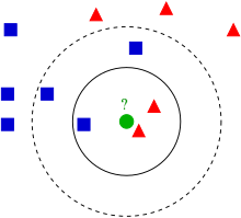 Example of k-NN classification. The test sample (green circle) should be classified either to the first class of blue squares or to the second class of red triangles. If k = 3(solid line circle) it is assigned to the second class because there are 2 triangles and only 1 square inside the inner circle. If k = 5(dashed line circle) it is assigned to the first class (3 squares vs. 2 triangles inside the outer circle). The training examples are vectors in a multidimensional feature space, each with a class label. The training phase of the algorithm consists only of storing the feature vectors and class labels of the training samples. In the classification phase, k is a user-defined constant, and an unlabeled vector (a query or test point) is classified by assigning the label which is most frequent among the k training samples nearest to that query point. A commonly used distance metric for continuous variables is Euclidean distance. For discrete variables, such as for text classification, another metric can be used, such as the overlap metric (or Hamming distance). Often, the classification accuracy of k-NN can be improved significantly if the distance metric is learned with specialized algorithms such as Large Margin Nearest Neighbor or Neighbourhood components analysis. A drawback of the basic "majority voting" classification occurs when the class distribution is skewed. That is, examples of a more frequent class tend to dominate the prediction of the new example, because they tend to be common among the k nearest neighbors due to their large number.[2] One way to overcome this problem is to weight the classification, taking into account the distance from the test point to each of itsk nearest neighbors. The class (or value, in regression problems) of each of the k nearest points is multiplied by a weight proportional to the inverse of the distance from that point to the test point. Another way to overcome skew is by abstraction in data representation. For example in a self-organizing map (SOM), each node is a representative (a center) of a cluster of similar points, regardless of their density in the original training data. KNN can then be applied to the SOM. Parameter selection[edit]The best choice of k depends upon the data; generally, larger values of k reduce the effect of noise on the classification,[3] but make boundaries between classes less distinct. A good k can be selected by various heuristic techniques (see hyperparameter optimization). The special case where the class is predicted to be the class of the closest training sample (i.e. when k = 1) is called the nearest neighbor algorithm. The accuracy of the k-NN algorithm can be severely degraded by the presence of noisy or irrelevant features, or if the feature scales are not consistent with their importance. Much research effort has been put into selecting or scaling features to improve classification. A particularly popular[citation needed] approach is the use of evolutionary algorithms to optimize feature scaling.[4] Another popular approach is to scale features by the mutual information of the training data with the training classes.[citation needed] In binary (two class) classification problems, it is helpful to choose k to be an odd number as this avoids tied votes. One popular way of choosing the empirically optimal k in this setting is via bootstrap method.[5] Properties[edit]KNN is a special case of a variable-bandwidth, kernel density "balloon" estimator with a uniform kernel.[6] [7] The naive version of the algorithm is easy to implement by computing the distances from the test example to all stored examples, but it is computationally intensive for large training sets. Using an appropriate nearest neighbor search algorithm makes kNN computationally tractable even for large data sets. Many nearest neighbor search algorithms have been proposed over the years; these generally seek to reduce the number of distance evaluations actually performed. kNN has some strong consistency results. As the amount of data approaches infinity, the algorithm is guaranteed to yield an error rate no worse than twice the Bayes error rate (the minimum achievable error rate given the distribution of the data).[8] KNN is guaranteed to approach the Bayes error rate for some value of k (where k increases as a function of the number of data points). Various improvements to kNN are possible by using proximity graphs.[9] When the input data to an algorithm is too large to be processed and it is suspected to be notoriously redundant (e.g. the same measurement in both feet and meters) then the input data will be transformed into a reduced representation set of features (also named features vector). Transforming the input data into the set of features is called Feature extraction. If the features extracted are carefully chosen it is expected that the features set will extract the relevant information from the input data in order to perform the desired task using this reduced representation instead of the full size input. Feature extraction is performed on raw data prior to applying K-NN algorithm on the transformed data in Feature space. An example of a typical Computer vision computation pipeline for face recognition using K-NN including feature extraction and dimension reduction pre-processing steps (usually implemented with OpenCV): 1. Haar face detection 2. Mean-shift tracking analysis 3. PCA or Fisher LDA projection into feature space, followed by K-NN classification Dimension reduction[edit]For high-dimensional data (e.g., with number of dimensions more than 10) dimension reduction is usually performed prior to applying the KNN algorithm in order to avoid the effects of thecurse of dimensionality. [10] The curse of dimensionality in the KNN context basically means that Euclidean distance is unhelpful in high dimensions because all vectors being are almost equidistant to the search query vector (imagine multiple points lying more or less on a circle of with the query point at the center; the distance from the query to all data points in the search space is almost the same). Feature extraction and dimension reduction can be combined in one step using principal component analysis (PCA), linear discriminant analysis (LDA), or canonical correlation analysis(CCA) techniques as a pre-processing step, followed by clustering by KNN on feature vectors in reduced-dimension space. In machine learning this process is also called low-dimensional embedding.[11] For very high-dimensional datasets (e.g. when performing a similarity search on live video streams, DNA data or high dimensional time series) running a fast approximate KNN search using locality sensitive hashing, "random projections",[12] "sketches" [13] or other high-dimensional similarity search techniques from VLDB toolbox might be the only feasible option. Data reduction[edit]Data reduction is one of the most important problems for work with huge data sets. Usually, only some of the data points are needed for accurate classification. Those data are called theprototypes and can be found as follows: - Select the class-outliers, that is, training data that are classified incorrectly by kNN (for a given k)
- Separate the rest of the data into two sets: (i) the prototypes that are used for the classification decisions and the absorbed points that can be correctly classified by kNN using prototypes and can be removed from the training set.
Selection of class-outliers[edit]A training example surrounded by examples of other classes is called a class outlier. Causes of class outliers include: - random error
- insufficient training examples of this class (an isolated example appears instead of a cluster)
- missing important features (the classes are separated in other dimensions which we do not know)
- too many training examples of other classes (unbalanced classes) that create a "hostile" background for the given small class
Class outliers with kNN produce noise. They can be detected and separated for future analysis. Given two natural numbers, k>r>0, a training example is called a (k,r)NN class-outlier if its k nearest neighbors include more than r examples of other classes. CNN for data reduction[edit]Condensed nearest neighbor (CNN, the Hart algorithm) is an algorithm designed to reduce the data set for kNN classification.[14] It selects the set of prototypes U from the training data, such that 1NN with U can classify the examples almost as accurately as 1NN does with the whole data set.  Calculation of the border ratio.  Three types of points: prototypes, class-outliers, and absorbed points. Given a training set X, CNN works iteratively: - Scan all elements of X, looking for an element x whose nearest prototype from U has a different label than x.
- Remove x from X and add it to U
- Repeat the scan until no more prototypes are added to U.
Use U instead of X for classification. The examples that are not prototypes are called "absorbed" points. It is efficient to scan the training examples in order of decreasing border ratio.[15] The border ratio of a training example x is defined as - a(x) = ||x'-y|| / ||x-y||
where ||x-y|| is the distance to the closest example y having a different color than x, and ||x'-y|| is the distance from y to its closest example x' with the same label as x. The border ratio is in the interval [0,1] because ||x'-y|| never exceeds ||x-y||. This ordering gives preference to the borders of the classes for inclusion in the set of prototypesU. A point of a different label than x is called external to x. The calculation of the border ratio is illustrated by the figure on the right. The data points are labeled by colors: the initial point is x and its label is red. External points are blue and green. The closest to x external point is y. The closest to yred point is x' . The border ratio a(x)=||x'-y||/||x-y|| is the attribute of the initial point x. Below is an illustration of CNN in a series of figures. There are three classes (red, green and blue). Fig. 1: initially there are 60 points in each class. Fig. 2 shows the 1NN classification map: each pixel is classified by 1NN using all the data. Fig. 3 shows the 5NN classification map. White areas correspond to the unclassified regions, where 5NN voting is tied (for example, if there are two green, two red and one blue points among 5 nearest neighbors). Fig. 4 shows the reduced data set. The crosses are the class-outliers selected by the (3,2)NN rule (all the three nearest neighbors of these instances belong to other classes); the squares are the prototypes, and the empty circles are the absorbed points. The left bottom corner shows the numbers of the class-outliers, prototypes and absorbed points for all three classes. The number of prototypes varies from 15% to 20% for different classes in this example. Fig. 5 shows that the 1NN classification map with the prototypes is very similar to that with the initial data set. The figures were produced using the Mirkes applet.[15] - CNN model reduction for KNN classifiers
-
-
Fig. 2. The 1NN classification map. -
Fig. 3. The 5NN classification map. -
Fig. 4. The CNN reduced dataset. -
Fig. 5. The 1NN classification map based on the CNN extracted prototypes. For regression[edit]The k-NN algorithm can also be adapted for regression, that is for estimating continuous variables. One such algorithm uses a weighted average of the k-nearest neighbors, weighted by the inverse of their distance. This algorithm is as follows: - Compute the Euclidean or Mahalanobis distance from the query example to the labeled examples.
- Order the labeled examples by increasing distance.
- Find a heuristically optimal number k of nearest neighbors, based on RMSE. This is done using cross validation.
- Calculate an inverse distance weighted average with the k-nearest multivariate neighbors.
Validation of results[edit]A confusion matrix or "matching matrix" is often used as a tool to validate the accuracy of K-NN classification. More robust statistical methods such as likelihood-ratio test can also be applied. See also[edit]References[edit] - Jump up^ Bremner D, Demaine E, Erickson J, Iacono J, Langerman S, Morin P, Toussaint G (2005). "Output-sensitive algorithms for computing nearest-neighbor decision boundaries". Discrete and Computational Geometry 33 (4): 593–604.doi:10.1007/s00454-004-1152-0.
- Jump up^ D. Coomans; D.L. Massart (1982). "Alternative k-nearest neighbour rules in supervised pattern recognition : Part 1. k-Nearest neighbour classification by using alternative voting rules". Analytica Chimica Acta 136: 15–27. doi:10.1016/S0003-2670(01)95359-0.
- Jump up^ Everitt, B. S., Landau, S., Leese, M. and Stahl, D. (2011) Miscellaneous Clustering Methods, in Cluster Analysis, 5th Edition, John Wiley & Sons, Ltd, Chichester, UK.
- Jump up^ Nigsch F, Bender A, van Buuren B, Tissen J, Nigsch E, Mitchell JB (2006). "Melting point prediction employing k-nearest neighbor algorithms and genetic parameter optimization".Journal of Chemical Information and Modeling 46 (6): 2412–2422.doi:10.1021/ci060149f. PMID 17125183.
- Jump up^ Hall P, Park BU, Samworth RJ (2008). "Choice of neighbor order in nearest-neighbor classification". Annals of Statistics 36 (5): 2135–2152. doi:10.1214/07-AOS537.
- Jump up^ D. G. Terrell; D. W. Scott (1992). "Variable kernel density estimation". Annals of Statistics20 (3): 1236–1265. doi:10.1214/aos/1176348768.
- Jump up^ Mills, Peter. "Efficient statistical classification of satellite measurements". International Journal of Remote Sensing.
- Jump up^ Cover TM, Hart PE (1967). "Nearest neighbor pattern classification". IEEE Transactions on Information Theory 13 (1): 21–27. doi:10.1109/TIT.1967.1053964.
- Jump up^ Toussaint GT (April 2005). "Geometric proximity graphs for improving nearest neighbor methods in instance-based learning and data mining". International Journal of Computational Geometry and Applications 15 (2): 101–150.doi:10.1142/S0218195905001622.
- Jump up^ Beyer, Kevin, et al.. 'When is “nearest neighbor” meaningful?. Database Theory—ICDT’99, 217-235|year 1999
- Jump up^ Shaw, Blake, and Tony Jebara. 'Structure preserving embedding. Proceedings of the 26th Annual International Conference on Machine Learning. ACM,2009
- Jump up^ Bingham, Ella, and Heikki Mannila. Random projection in dimensionality reduction: applications to image and text data. Proceedings of the seventh ACM SIGKDD international conference on Knowledge discovery and data mining. ACM | year 2001
- Jump up^ Shasha, D High Performance Discovery in Time Series.Berlin: Springer, 2004, ISBN 0-387-00857-8
- Jump up^ P. E. Hart, The Condensed Nearest Neighbor Rule. IEEE Transactions on Information Theory 18 (1968) 515–516. doi: 10.1109/TIT.1968.1054155
- ^ Jump up to:a b E. M. Mirkes, KNN and Potential Energy: applet. University of Leicester, 2011.
Further reading[edit] |
+Citations (1) - CitationsAdd new citationList by: CiterankMapLink[1] Wikipedia
Author: Various
Cited by: Roger Yau 2:28 PM 21 October 2013 GMT
Citerank: (28) 291862AODE - Averaged one-dependence estimatorsAveraged one-dependence estimators (AODE) is a probabilistic classification learning technique. It was developed to address the attribute-independence problem of the popular naive Bayes classifier. It frequently develops substantially more accurate classifiers than naive Bayes at the cost of a modest increase in the amount of computation.109FDEF6, 291863Artificial neural networkIn computer science and related fields, artificial neural networks are computational models inspired by animal central nervous systems (in particular the brain) that are capable of machine learning and pattern recognition. They are usually presented as systems of interconnected "neurons" that can compute values from inputs by feeding information through the network.109FDEF6, 291936BackpropagationBackpropagation, an abbreviation for "backward propagation of errors", is a common method of training artificial neural networks. From a desired output, the network learns from many inputs, similar to the way a child learns to identify a dog from examples of dogs.109FDEF6, 291937Bayesian statisticsBayesian statistics is a subset of the field of statistics in which the evidence about the true state of the world is expressed in terms of degrees of belief or, more specifically, Bayesian probabilities. Such an interpretation is only one of a number of interpretations of probability and there are other statistical techniques that are not based on "degrees of belief".109FDEF6, 291938Naive Bayes classifierA naive Bayes classifier is a simple probabilistic classifier based on applying Bayes' theorem with strong (naive) independence assumptions. A more descriptive term for the underlying probability model would be "independent feature model". An overview of statistical classifiers is given in the article on Pattern recognition.109FDEF6, 291939Bayesian networkA Bayesian network, Bayes network, belief network, Bayes(ian) model or probabilistic directed acyclic graphical model is a probabilistic graphical model (a type of statistical model) that represents a set of random variables and their conditional dependencies via a directed acyclic graph (DAG). For example, a Bayesian network could represent the probabilistic relationships between diseases and symptoms. 109FDEF6, 291941Case-based reasoningCase-based reasoning (CBR), broadly construed, is the process of solving new problems based on the solutions of similar past problems. An auto mechanic who fixes an engine by recalling another car that exhibited similar symptoms is using case-based reasoning. So, too, an engineer copying working elements of nature (practicing biomimicry), is treating nature as a database of solutions to problems. Case-based reasoning is a prominent kind of analogy making.109FDEF6, 291942Decision tree learningDecision tree learning uses a decision tree as a predictive model which maps observations about an item to conclusions about the item's target value. It is one of the predictive modelling approaches used in statistics, data mining and machine learning. More descriptive names for such tree models are classification trees or regression trees. In these tree structures, leaves represent class labels and branches represent conjunctions of features that lead to those class labels.109FDEF6, 291943Inductive logic programmingInductive logic programming (ILP) is a subfield of machine learning which uses logic programming as a uniform representation for examples, background knowledge and hypotheses. Given an encoding of the known background knowledge and a set of examples represented as a logical database of facts, an ILP system will derive a hypothesised logic program which entails all the positive and none of the negative examples.109FDEF6, 291944Gaussian process regression (Kriging)Kriging is a method to build an approximation of a function from a set of evaluations of the function at a finite set of points. The method originates from the domain of geostatistics and is now widely used in the domain of spatial analysis and computer experiments. The technique is also known as Gaussian process regression, Kolmogorov Wiener prediction, or Best Linear Unbiased Prediction.109FDEF6, 291945Gene expression programmingGene expression programming (GEP) is an evolutionary algorithm that creates computer programs or models. These computer programs are complex tree structures that learn and adapt by changing their sizes, shapes, and composition, much like a living organism. And like living organisms, the computer programs of GEP are also encoded in simple linear chromosomes of fixed length. Thus, GEP is a genotype-phenotype system.109FDEF6, 291946Group method of data handlingGroup method of data handling (GMDH) is a family of inductive algorithms for computer-based mathematical modeling of multi-parametric datasets that features fully automatic structural and parametric optimization of models.109FDEF6, 291947Learning automataA branch of the theory of adaptive control is devoted to learning automata surveyed by Narendra and Thathachar which were originally described explicitly as finite state automata. Learning automata select their current action based on past experiences from the environment.109FDEF6, 291948Supervised learningSupervised learning is the machine learning task of inferring a function from labeled training data.[1] The training data consist of a set of training examples. In supervised learning, each example is a pair consisting of an input object (typically a vector) and a desired output value (also called the supervisory signal). A supervised learning algorithm analyzes the training data and produces an inferred function, which can be used for mapping new examples. 25CBCBFF, 291950Unsupervised learningIn machine learning, the problem of unsupervised learning is that of trying to find hidden structure in unlabeled data. Since the examples given to the learner are unlabeled, there is no error or reward signal to evaluate a potential solution. This distinguishes unsupervised learning from supervised learning and reinforcement learning.25CBCBFF, 291951Reinforcement learningReinforcement learning is an area of machine learning inspired by behaviorist psychology, concerned with how software agents ought to take actions in an environment so as to maximize some notion of cumulative reward. The problem, due to its generality, is studied in many other disciplines, such as game theory, control theory, operations research, information theory, simulation-based optimization, statistics, and genetic algorithms.25CBCBFF, 292450Hierarchical clusteringIn data mining, hierarchical clustering is a method of cluster analysis which seeks to build a hierarchy of clusters. Strategies for hierarchical clustering generally fall into two types:
Agglomerative: This is a "bottom up" approach: each observation starts in its own cluster, and pairs of clusters are merged as one moves up the hierarchy.
Divisive: This is a "top down" approach: all observations start in one cluster, and splits are performed recursively as one moves down the hierarch109FDEF6, 292451Association rule learningAssociation rule learning is a popular and well researched method for discovering interesting relations between variables in large databases. It is intended to identify strong rules discovered in databases using different measures of interestingness.109FDEF6, 292454Others25CBCBFF, 292455Learning Vector QuantizationIn computer science, Learning Vector Quantization (LVQ), is a prototype-based supervised classification algorithm. LVQ is the supervised counterpart of vector quantization systems.
LVQ can be understood as a special case of an artificial neural network, more precisely, it applies a winner-take-all Hebbian learning-based approach. It is a precursor to Self-organizing maps (SOM) and related to Neural gas, and to the k-Nearest Neighbor algorithm (k-NN). LVQ was invented by Teuvo Kohonen.109FDEF6, 292463Logistic Model TreeLMT is a classification model with an associated supervised training algorithm that combines logistic regression (LR) and decision tree learning. Logistic model trees are based on the earlier idea of a model tree: a decision tree that has linear regression models at its leaves to provide a piecewise linear regression model (where ordinary decision trees with constants at their leaves would produce a piecewise constant model).109FDEF6, 292464Minimum message lengthMinimum message length (MML) is a formal information theory restatement of Occam's Razor: even when models are not equal in goodness of fit accuracy to the observed data, the one generating the shortest overall message is more likely to be correct (where the message consists of a statement of the model, followed by a statement of data encoded concisely using that model). MML was invented by Chris Wallace, first appearing in the seminal (Wallace and Boulton, 1968).109FDEF6, 292465Lazy learningIn artificial intelligence, lazy learning is a learning method in which generalization beyond the training data is delayed until a query is made to the system, as opposed to in eager learning, where the system tries to generalize the training data before receiving queries.109FDEF6, 292466Instance-based learninginstance-based learning or memory-based learning is a family of learning algorithms that, instead of performing explicit generalization, compare new problem instances with instances seen in training, which have been stored in memory. Instance-based learning is a kind of lazy learning.109FDEF6, 292476Analogical modelingAnalogical modeling (hereafter AM) is a formal theory of exemplar-based analogical reasoning, proposed by Royal Skousen, professor of Linguistics and English language at Brigham Young University in Provo, Utah. It is applicable to language modeling and other categorization tasks. Analogical modeling is related to connectionism and nearest neighbor approaches, in that it is data-based rather than abstraction-based.109FDEF6, 292478Probably approximately correct learningIn this framework, the learner receives samples and must select a generalization function (called the hypothesis) from a certain class of possible functions. The goal is that, with high probability (the "probably" part), the selected function will have low generalization error (the "approximately correct" part). The learner must be able to learn the concept given any arbitrary approximation ratio, probability of success, or distribution of the samples.109FDEF6, 292480Ripple-down rulesRipple Down Rules is a way of approaching knowledge acquisition. Knowledge acquisition refers to the transfer of knowledge from human experts to knowledge based systems.109FDEF6, 292481Support vector machinesIn machine learning, support vector machines (SVMs, also support vector networks[1]) are supervised learning models with associated learning algorithms that analyze data and recognize patterns, used for classification and regression analysis. 109FDEF6 URL: |
|
|