|
![]()
| Gaussian process regression (Kriging) Component1 #291944 Kriging is a method to build an approximation of a function from a set of evaluations of the function at a finite set of points. The method originates from the domain of geostatistics and is now widely used in the domain of spatial analysis and computer experiments. The technique is also known as Gaussian process regression, Kolmogorov Wiener prediction, or Best Linear Unbiased Prediction. | Kriging is a method to build an approximation of a function from a set of evaluations of the function at a finite set of points. The method originates from the domain of geostatistics and is now widely used in the domain of spatial analysis and computer experiments. The technique is also known as Gaussian process regression, Kolmogorov Wiener prediction, orBest Linear Unbiased Prediction.  Example of one-dimensional data interpolation by kriging, with confidence intervals. Squares indicate the location of the data. The kriging interpolation is in red. The confidence intervals are represented by gray areas. The theory behind interpolating or extrapolating by kriging was developed by the French mathematicianGeorges Matheron based on the Master's thesis of Danie G. Krige, the pioneering plotter of distance-weighted average gold grades at the Witwatersrand reef complex in South Africa. The English verb is to krige and the most common noun is kriging; both are often pronounced with a hard "g", following the pronunciation of the name "Krige". Contents [hide] - 1 Main principles
- 1.1 Related terms and techniques
- 1.2 Geostatistical estimator
- 1.3 Linear estimation
- 2 Methods
- 2.1 Ordinary kriging
- 2.2 Simple kriging
- 2.2.1 Kriging system
- 2.2.2 Estimation
- 2.3 Properties
- 3 Applications
- 3.1 Design and analysis of computer experiments
- 4 See also
- 5 References
- 5.1 Books
- 5.2 Historical references
- 5.3 Software related to kriging
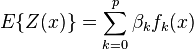
Main principles[edit]Related terms and techniques[edit]The basic idea of kriging to predict the value of a function at a given point by computing a weighted average of the known values of the function in the neighborhood of the point. The method is mathematically closely related to regression analysis. Both theories derive a best linear unbiased estimator, based on assumptions on covariances, make use of Gauss-Markov theorem to prove independence of the estimate and error, and make use of very similar formulae. They are nevertheless, useful in different frameworks: kriging is made for estimation of a single realization of a random field, while regression models are based on multiple observations of a multivariate dataset. The kriging estimation may also be seen as a spline in a reproducing kernel Hilbert space, with reproducing kernel given by the covariance function.[1] The difference with the classical kriging approach is provided by the interpretation: while the spline is motivated by a minimum norm interpolation based on a Hilbert space structure, kriging is motivated by an expected squared prediction error based on a stochastic model. Kriging with polynomial trend surfaces is mathematically identical to generalized least squares polynomial curve fitting. Kriging can also be understood as a form of Bayesian inference.[2] Kriging starts with a prior distribution over functions. This prior takes the form of a Gaussian process:  samples from a function will be normally distributed, where the covariance between any two samples is the covariance function (or kernel) of the Gaussian process evaluated at the spatial location of two points. A set of values is then observed, each value associated with a spatial location. Now, a new value can be predicted at any new spatial location, by combining the Gaussian prior with a Gaussian likelihood function for each of the observed values. The resulting posterior distribution is also Gaussian, with a mean and covariance that can be simply computed from the observed values, their variance, and the kernel matrix derived from the prior. samples from a function will be normally distributed, where the covariance between any two samples is the covariance function (or kernel) of the Gaussian process evaluated at the spatial location of two points. A set of values is then observed, each value associated with a spatial location. Now, a new value can be predicted at any new spatial location, by combining the Gaussian prior with a Gaussian likelihood function for each of the observed values. The resulting posterior distribution is also Gaussian, with a mean and covariance that can be simply computed from the observed values, their variance, and the kernel matrix derived from the prior. Geostatistical estimator[edit]In geostatistical models, sampled data is interpreted as a result of a random process. The fact that this models incorporate uncertainty in its conceptualization doesn't mean that the phenomenon - the forest, the aquifer, the mineral deposit - has resulted from a random process, but solely allows to build a methodological basis for the spatial inference of quantities in unobserved locations and to the quantification of the uncertainty associated with the estimator. A stochastic process is simply, in the context of this model, a way to approach the set of data collected from the samples. The first step in geostatistical modulation is the creation of a random process that best describes the set of experimental observed data.[3] A value spatially located at  (generic denomination of a set of geographic coordinates) is interpreted as a realization (generic denomination of a set of geographic coordinates) is interpreted as a realization  of the random variable of the random variable  . In the space . In the space  , where the set of samples is dispersed, exists realizations of the random variables , where the set of samples is dispersed, exists realizations of the random variables  , correlated between themselves. , correlated between themselves. The set of random variables, constitutes a random function of which only one realization is known  - the set of experimental data. With only one realization of each random variable it's theoretically impossible to determine any statistical parameter of the individual variables or the function. - the set of experimental data. With only one realization of each random variable it's theoretically impossible to determine any statistical parameter of the individual variables or the function. - The proposed solution in the geostatistical formalism consists in assuming various degrees of stationarity in the random function, in order to make possible the inference of some statistic values.[4]
For instance, if a workgroup of scientists assumes appropriate, based on the homogeneity of samples in area where the variable is distributed, the hypothesis that the first moment is stationary (i.e. all random variables have the same mean), than, they are implying that the mean can be estimated by the arithmetic mean of sampled values. Judging an hypothesis like this as appropriate is the same as considering that sample values are sufficiently homogeneous to validate that representativity. The hypothesis of stationarity related to the second moment is defined in the following way: the correlation between two random variables solely depends on the spatial distance that separates them and is independent of its location:   where  This hypothesis allows to infer those two measures - the variogram and the covariogram - based on the samples:  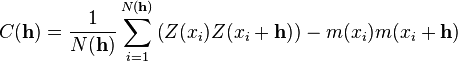 where 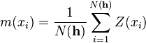 Linear estimation[edit]Spatial inference, or estimation, of a quantity  , at an unobserved location , at an unobserved location  , is calculated from a linear combination of the observed values , is calculated from a linear combination of the observed values  and weights and weights 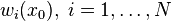 : : 
The weights  are intended to summarize two extremely important procedures in a spatial inference process: are intended to summarize two extremely important procedures in a spatial inference process: - reflect the structural "proximity" of samples to the estimation location,
- at the same time, they should have a desegregation effect, in order to avoid bias caused by eventual sample clusters
When calculating the weights , there are two objectives in the geostatistical formalism: unbias and minimal variance of estimation. If the cloud of real values  is plotted against the estimated values is plotted against the estimated values  , the criterion for global unbias, intrinsic stationarity or wide sense stationarity of the field, implies that the mean of the estimations must be equal to mean of the real values. , the criterion for global unbias, intrinsic stationarity or wide sense stationarity of the field, implies that the mean of the estimations must be equal to mean of the real values. The second criterion says that the mean of the squared deviations  must be minimal, what means that when the cloud of estimated values versus the cloud real values is more disperse, more imprecise the estimator is. must be minimal, what means that when the cloud of estimated values versus the cloud real values is more disperse, more imprecise the estimator is. Methods[edit]Depending on the stochastic properties of the random field and the various degrees of stationarity assumed, different methods for calculating the weights can be deducted, i.e. different types of kriging apply. Classical methods are: - Ordinary kriging assumes stationarity of the first moment of all random variables:
 , where , where  is unknown. is unknown. - Simple kriging assumes a known stationary mean:
 , where is known. , where is known. - Universal kriging assumes a general polynomial trend model, such as linear trend model
 . . - IRFk-kriging assumes
 to be an unknown polynomial in to be an unknown polynomial in  . . - Indicator kriging uses indicator functions instead of the process itself, in order to estimate transition probabilities.
- Multiple-indicator kriging is a version of indicator kriging working with a family of indicators. However, MIK has fallen out of favour as an interpolation technique in recent years. This is due to some inherent difficulties related to operation and model validation. Conditional simulation is fast becoming the accepted replacement technique in this case.
- Disjunctive kriging is a nonlinear generalisation of kriging.
- Lognormal kriging interpolates positive data by means of logarithms.
Ordinary kriging[edit]The unknown value is interpreted as a random variable located in , as well as the values of neighbors samples  . The estimator is also interpreted as a random variable located in , a result of the linear combination of variables. . The estimator is also interpreted as a random variable located in , a result of the linear combination of variables. In order to deduce the kriging system for the assumptions of the model, the following error committed while estimating  in is declared: in is declared:  The two quality criteria referred previously can now be expressed in terms of the mean and variance of the new random variable  : : Unbias Since the random function is stationary,  , the following constraint is observed: , the following constraint is observed:   In order to ensure that the model is unbiased, the sum of weights needs to be one. Minimal Variance: minimize  Two estimators can have  , but the dispersion around their mean determines the difference between the quality of estimators. , but the dispersion around their mean determines the difference between the quality of estimators.  * see covariance matrix for a detailed explanation 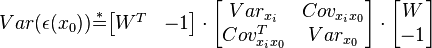 * where the literals  stand for stand for  . . Once defined the covariance model or variogram,  or or  , valid in all field of analysis of , than we can write an expression for the estimation variance of any estimator in function of the covariance between the samples and the covariances between the samples and the point to estimate: , valid in all field of analysis of , than we can write an expression for the estimation variance of any estimator in function of the covariance between the samples and the covariances between the samples and the point to estimate:  Some conclusions can be asserted from this expressions. The variance of estimation: - is not quantifiable to any linear estimator, once the stationarity of the mean and of the spatial covariances, or variograms, are assumed.
- grows with the covariance between samples
 , i.e. to the same distance to the estimating point, if the samples are proximal to each other, than the clustering effect, or informational redundancy, is bigger, so the estimation is worst. This conclusion is valid to any value of the weights: a preferential grouping of samples is always worst, which means that for the same number of samples the estimation variance grows with the relative weight of the sample clusters. , i.e. to the same distance to the estimating point, if the samples are proximal to each other, than the clustering effect, or informational redundancy, is bigger, so the estimation is worst. This conclusion is valid to any value of the weights: a preferential grouping of samples is always worst, which means that for the same number of samples the estimation variance grows with the relative weight of the sample clusters. - grows when the covariance between the samples and the point to estimate decreases. This means that, when the samples are more far away from , the worst is the estimation.
- grows with the a priori variance
 of the variable . When the variable is less disperse, the variance is lower in any point of the area . of the variable . When the variable is less disperse, the variance is lower in any point of the area . - does not depend on the values of the samples. This means that the same spatial configuration (with the same geometrical relations between samples and the point to estimate) always reproduces the same estimation variance in any part of the area . This way, the variance does not measures the uncertainty of estimation produced by the local variable.
Kriging system[edit]  Solving this optimization problem (see Lagrange multipliers) results in the kriging system: 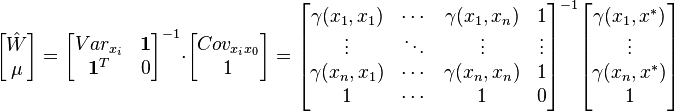 the additional parameter  is a Lagrange multiplier used in the minimization of the kriging error is a Lagrange multiplier used in the minimization of the kriging error  to honor the unbiasedness condition. to honor the unbiasedness condition. Simple kriging[edit]Simple kriging is mathematically the simplest, but the least general. It assumes the expectation of the random field to be known, and relies on a covariance function. However, in most applications neither the expectation nor the covariance are known beforehand. The practical assumptions for the application of simple kriging are: Kriging system[edit]The kriging weights of simple kriging have no unbiasedness condition and are given by the simple kriging equation system: 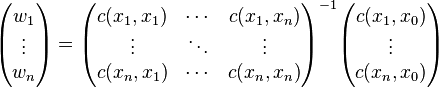 This is analogous to a linear regression of on the other  . . Estimation[edit]The interpolation by simple kriging is given by:  The kriging error is given by:  which leads to the generalised least squares version of the Gauss-Markov theorem (Chiles & Delfiner 1999, p. 159):  Properties[edit](Cressie 1993, Chiles&Delfiner 1999, Wackernagel 1995) - The kriging estimation is unbiased:
![E[\hat{Z}(x_i)]=E[Z(x_i)]](http://upload.wikimedia.org/math/3/d/7/3d7251d06e9bc6964ec3d65807950fe6.png) - The kriging estimation honors the actually observed value:
 (assuming no measurement error is incurred) (assuming no measurement error is incurred) - The kriging estimation
 is the best linear unbiased estimator of if the assumptions hold. However (e.g. Cressie 1993): is the best linear unbiased estimator of if the assumptions hold. However (e.g. Cressie 1993): - As with any method: If the assumptions do not hold, kriging might be bad.
- There might be better nonlinear and/or biased methods.
- No properties are guaranteed, when the wrong variogram is used. However typically still a 'good' interpolation is achieved.
- Best is not necessarily good: e.g. In case of no spatial dependence the kriging interpolation is only as good as the arithmetic mean.
- Kriging provides
 as a measure of precision. However this measure relies on the correctness of the variogram. as a measure of precision. However this measure relies on the correctness of the variogram. Applications[edit]Although kriging was developed originally for applications in geostatistics, it is a general method of statistical interpolation that can be applied within any discipline to sampled data from random fields that satisfy the appropriate mathematical assumptions. To date kriging has been used in a variety of disciplines, including the following: and many others. Design and analysis of computer experiments[edit]Another very important and rapidly growing field of application, in engineering, is the interpolation of data coming out as response variables of deterministic computer simulations,[16] e.g.finite element method (FEM) simulations. In this case, kriging is used as a metamodeling tool, i.e. a black box model built over a designed set of computer experiments. In many practical engineering problems, such as the design of a metal forming process, a single FEM simulation might be several hours or even a few days long. It is therefore more efficient to design and run a limited number of computer simulations, and then use a kriging interpolator to rapidly predict the response in any other design point. Kriging is therefore used very often as a so-called surrogate model, implemented inside optimization routines.[17] See also[edit]References[edit] - Jump up^ Grace Wahba (1990). Spline Models for Observational Data 59. SIAM. p. 162.
- Jump up^ Williams, Christopher K.I. (1998). "Prediction with Gaussian processes: From linear regression to linear prediction and beyond". In M. I. Jordan. Learning in graphical models. MIT Press. pp. 599–612.
- Jump up^ Soares 2006, p.18
- Jump up^ Matheron G. 1978
- Jump up^ Hanefi Bayraktar and F. Sezer. Turalioglu (2005) "A Kriging-based approach for locating a sampling site—in the assessment of air quality, SERRA, 19 (4), 301-305 doi:10.1007/s00477-005-0234-8
- Jump up^ Chiles, J.-P. and P. Delfiner (1999) Geostatistics, Modeling Spatial Uncertainty, Wiley Series in Probability and statistics.
- Jump up^ Zimmerman, D.A. et al. (1998) "A comparison of seven geostatistically based inverse approaches to estimate transmissivies for modelling advective transport by groundwater flow", Water Resources Research, 34 (6), 1273-1413
- Jump up^ Tonkin M.J. Larson (2002) "Kriging Water Levels with a Regional-Linear and Point Logarithmic Drift", Ground Water, 33 (1), 338-353,
- Jump up^ Journel, A.G. and C.J. Huijbregts (1978) Mining Geostatistics, Academic Press London
- Jump up^ Andrew Richmond (2003) "Financially Efficient Ore Selection Incorporating Grade Uncertainty", Mathematical Geology, 35 (2), 195-215
- Jump up^ Goovaerts (1997) Geostatistics for natural resource evaluation, OUP. ISBN 0-19-511538-4
- Jump up^ X. Emery (2005) "Simple and Ordinary Kriging Multigaussian Kriging for Estimating recoverarble Reserves", Mathematical Geology, 37 (3), 295-31)
- Jump up^ A. Stein, F. van der Meer, B. Gorte (Eds.) (2002) Spatial Statistics for remote sensing. Springer. ISBN 0-7923-5978-X
- Jump up^ Barris, J. (2008) An expert system for appraisal by the method of comparison. PhD Thesis, UPC, Barcelona
- Jump up^ Barris, J. and Garcia Almirall,P.(2010) A density function of the appraisal value., UPC, Barcelona
- Jump up^ Sacks, J. and Welch, W.J. and Mitchell, T.J. and Wynn, H.P. (1989). Design and Analysis of Computer Experiments 4 (4). Statistical Science. pp. 409–435.
- Jump up^ Strano, M. (2008). "A technique for FEM optimization under reliability constraint of process variables in sheet metal forming". International Journal of Material Forming 1: 13–20.doi:10.1007/s12289-008-0001-8. edit
- Abramowitz, M., and Stegun, I. (1972), Handbook of Mathematical Functions, Dover Publications, New York.
- Banerjee, S., Carlin, B.P. and Gelfand, A.E. (2004). Hierarchical Modeling and Analysis for Spatial Data. Chapman and Hall/CRC Press, Taylor and Francis Group.
- Chiles, J.-P. and P. Delfiner (1999) Geostatistics, Modeling Spatial uncertainty, Wiley Series in Probability and statistics.
- Cressie, N (1993) Statistics for spatial data, Wiley, New York
- David, M (1988) Handbook of Applied Advanced Geostatistical Ore Reserve Estimation, Elsevier Scientific Publishing
- Deutsch, C.V., and Journel, A. G. (1992), GSLIB - Geostatistical Software Library and User's Guide, Oxford University Press, New York, 338 pp.
- Goovaerts, P. (1997) Geostatistics for Natural Resources Evaluation, Oxford University Press, New York ISBN 0-19-511538-4
- Isaaks, E. H., and Srivastava, R. M. (1989), An Introduction to Applied Geostatistics, Oxford University Press, New York, 561 pp.
- Journel, A. G. and C. J. Huijbregts (1978) Mining Geostatistics, Academic Press London
- Journel, A. G. (1989), Fundamentals of Geostatistics in Five Lessons, American Geophysical Union, Washington D.C.
- Press, WH; Teukolsky, SA; Vetterling, WT; Flannery, BP (2007), "Section 3.7.4. Interpolation by Kriging", Numerical Recipes: The Art of Scientific Computing (3rd ed.), New York: Cambridge University Press, ISBN 978-0-521-88068-8. Also, "Section 15.9. Gaussian Process Regression".
- Soares, A. (2000), Geoestatística para as Ciências da Terra e do Ambiente, IST Press, Lisbon, ISBN 972-8469-46-2
- Stein, M. L. (1999), Statistical Interpolation of Spatial Data: Some Theory for Kriging, Springer, New York.
- Wackernagel, H. (1995) Multivariate Geostatistics - An Introduction with Applications, Springer Berlin
Historical references[edit] - Agterberg, F P, Geomathematics, Mathematical Background and Geo-Science Applications, Elsevier Scientific Publishing Company, Amsterdam, 1974
- Cressie, N. A. C., The Origins of Kriging, Mathematical Geology, v. 22, pp 239–252, 1990
- Krige, D.G, A statistical approach to some mine valuations and allied problems at the Witwatersrand, Master's thesis of the University of Witwatersrand, 1951
- Link, R F and Koch, G S, Experimental Designs and Trend-Surface Analsysis, Geostatistics, A colloquium, Plenum Press, New York, 1970
- Matheron, G., "Principles of geostatistics", Economic Geology, 58, pp 1246–1266, 1963
- Matheron, G., "The intrinsic random functions, and their applications", Adv. Appl. Prob., 5, pp 439–468, 1973
- Merriam, D F, Editor, Geostatistics, a colloquium, Plenum Press, New York, 1970
Software related to kriging[edit] - BACCO - Bayesian analysis of computer code software
- tgp - Treed Gaussian processes
- DiceDesign, DiceEval, DiceKriging, DiceOptim - metamodeling packages of the Dice Consortium.
- DACE - Design and Analysis of Computer Experiments. A matlab kriging toolbox.
- GPML - Gaussian Processes for Machine Learning.
- STK - Small (Matlab/GNU Octave) Toolbox for Kriging for design and analysis of computer experiments.
- scalaGAUSS - Matlab kriging toolbox with a focus on large datasets
- DACE-Scilab - Scilab port of the DACE kriging matlab toolbox
- krigeage - Kriging toolbox for Scilab
- KRISP - Kriging based regression and optimization package for Scilab
- scikit-learn - machine learning in Python
|
+Citations (1) - CitationsAdd new citationList by: CiterankMapLink[1] Wikipedia
Author: Various
Cited by: Roger Yau 5:34 PM 19 October 2013 GMT
Citerank: (28) 291862AODE - Averaged one-dependence estimatorsAveraged one-dependence estimators (AODE) is a probabilistic classification learning technique. It was developed to address the attribute-independence problem of the popular naive Bayes classifier. It frequently develops substantially more accurate classifiers than naive Bayes at the cost of a modest increase in the amount of computation.109FDEF6, 291863Artificial neural networkIn computer science and related fields, artificial neural networks are computational models inspired by animal central nervous systems (in particular the brain) that are capable of machine learning and pattern recognition. They are usually presented as systems of interconnected "neurons" that can compute values from inputs by feeding information through the network.109FDEF6, 291936BackpropagationBackpropagation, an abbreviation for "backward propagation of errors", is a common method of training artificial neural networks. From a desired output, the network learns from many inputs, similar to the way a child learns to identify a dog from examples of dogs.109FDEF6, 291937Bayesian statisticsBayesian statistics is a subset of the field of statistics in which the evidence about the true state of the world is expressed in terms of degrees of belief or, more specifically, Bayesian probabilities. Such an interpretation is only one of a number of interpretations of probability and there are other statistical techniques that are not based on "degrees of belief".109FDEF6, 291938Naive Bayes classifierA naive Bayes classifier is a simple probabilistic classifier based on applying Bayes' theorem with strong (naive) independence assumptions. A more descriptive term for the underlying probability model would be "independent feature model". An overview of statistical classifiers is given in the article on Pattern recognition.109FDEF6, 291939Bayesian networkA Bayesian network, Bayes network, belief network, Bayes(ian) model or probabilistic directed acyclic graphical model is a probabilistic graphical model (a type of statistical model) that represents a set of random variables and their conditional dependencies via a directed acyclic graph (DAG). For example, a Bayesian network could represent the probabilistic relationships between diseases and symptoms. 109FDEF6, 291941Case-based reasoningCase-based reasoning (CBR), broadly construed, is the process of solving new problems based on the solutions of similar past problems. An auto mechanic who fixes an engine by recalling another car that exhibited similar symptoms is using case-based reasoning. So, too, an engineer copying working elements of nature (practicing biomimicry), is treating nature as a database of solutions to problems. Case-based reasoning is a prominent kind of analogy making.109FDEF6, 291942Decision tree learningDecision tree learning uses a decision tree as a predictive model which maps observations about an item to conclusions about the item's target value. It is one of the predictive modelling approaches used in statistics, data mining and machine learning. More descriptive names for such tree models are classification trees or regression trees. In these tree structures, leaves represent class labels and branches represent conjunctions of features that lead to those class labels.109FDEF6, 291943Inductive logic programmingInductive logic programming (ILP) is a subfield of machine learning which uses logic programming as a uniform representation for examples, background knowledge and hypotheses. Given an encoding of the known background knowledge and a set of examples represented as a logical database of facts, an ILP system will derive a hypothesised logic program which entails all the positive and none of the negative examples.109FDEF6, 291945Gene expression programmingGene expression programming (GEP) is an evolutionary algorithm that creates computer programs or models. These computer programs are complex tree structures that learn and adapt by changing their sizes, shapes, and composition, much like a living organism. And like living organisms, the computer programs of GEP are also encoded in simple linear chromosomes of fixed length. Thus, GEP is a genotype-phenotype system.109FDEF6, 291946Group method of data handlingGroup method of data handling (GMDH) is a family of inductive algorithms for computer-based mathematical modeling of multi-parametric datasets that features fully automatic structural and parametric optimization of models.109FDEF6, 291947Learning automataA branch of the theory of adaptive control is devoted to learning automata surveyed by Narendra and Thathachar which were originally described explicitly as finite state automata. Learning automata select their current action based on past experiences from the environment.109FDEF6, 291948Supervised learningSupervised learning is the machine learning task of inferring a function from labeled training data.[1] The training data consist of a set of training examples. In supervised learning, each example is a pair consisting of an input object (typically a vector) and a desired output value (also called the supervisory signal). A supervised learning algorithm analyzes the training data and produces an inferred function, which can be used for mapping new examples. 25CBCBFF, 291950Unsupervised learningIn machine learning, the problem of unsupervised learning is that of trying to find hidden structure in unlabeled data. Since the examples given to the learner are unlabeled, there is no error or reward signal to evaluate a potential solution. This distinguishes unsupervised learning from supervised learning and reinforcement learning.25CBCBFF, 291951Reinforcement learningReinforcement learning is an area of machine learning inspired by behaviorist psychology, concerned with how software agents ought to take actions in an environment so as to maximize some notion of cumulative reward. The problem, due to its generality, is studied in many other disciplines, such as game theory, control theory, operations research, information theory, simulation-based optimization, statistics, and genetic algorithms.25CBCBFF, 292450Hierarchical clusteringIn data mining, hierarchical clustering is a method of cluster analysis which seeks to build a hierarchy of clusters. Strategies for hierarchical clustering generally fall into two types:
Agglomerative: This is a "bottom up" approach: each observation starts in its own cluster, and pairs of clusters are merged as one moves up the hierarchy.
Divisive: This is a "top down" approach: all observations start in one cluster, and splits are performed recursively as one moves down the hierarch109FDEF6, 292451Association rule learningAssociation rule learning is a popular and well researched method for discovering interesting relations between variables in large databases. It is intended to identify strong rules discovered in databases using different measures of interestingness.109FDEF6, 292454Others25CBCBFF, 292455Learning Vector QuantizationIn computer science, Learning Vector Quantization (LVQ), is a prototype-based supervised classification algorithm. LVQ is the supervised counterpart of vector quantization systems.
LVQ can be understood as a special case of an artificial neural network, more precisely, it applies a winner-take-all Hebbian learning-based approach. It is a precursor to Self-organizing maps (SOM) and related to Neural gas, and to the k-Nearest Neighbor algorithm (k-NN). LVQ was invented by Teuvo Kohonen.109FDEF6, 292463Logistic Model TreeLMT is a classification model with an associated supervised training algorithm that combines logistic regression (LR) and decision tree learning. Logistic model trees are based on the earlier idea of a model tree: a decision tree that has linear regression models at its leaves to provide a piecewise linear regression model (where ordinary decision trees with constants at their leaves would produce a piecewise constant model).109FDEF6, 292464Minimum message lengthMinimum message length (MML) is a formal information theory restatement of Occam's Razor: even when models are not equal in goodness of fit accuracy to the observed data, the one generating the shortest overall message is more likely to be correct (where the message consists of a statement of the model, followed by a statement of data encoded concisely using that model). MML was invented by Chris Wallace, first appearing in the seminal (Wallace and Boulton, 1968).109FDEF6, 292465Lazy learningIn artificial intelligence, lazy learning is a learning method in which generalization beyond the training data is delayed until a query is made to the system, as opposed to in eager learning, where the system tries to generalize the training data before receiving queries.109FDEF6, 292466Instance-based learninginstance-based learning or memory-based learning is a family of learning algorithms that, instead of performing explicit generalization, compare new problem instances with instances seen in training, which have been stored in memory. Instance-based learning is a kind of lazy learning.109FDEF6, 292475k-nearest neighbor algorithmIn pattern recognition, the k-nearest neighbor algorithm (k-NN) is a non-parametric method for classifying objects based on closest training examples in the feature space. k-NN is a type of instance-based learning, or lazy learning where the function is only approximated locally and all computation is deferred until classification. 109FDEF6, 292476Analogical modelingAnalogical modeling (hereafter AM) is a formal theory of exemplar-based analogical reasoning, proposed by Royal Skousen, professor of Linguistics and English language at Brigham Young University in Provo, Utah. It is applicable to language modeling and other categorization tasks. Analogical modeling is related to connectionism and nearest neighbor approaches, in that it is data-based rather than abstraction-based.109FDEF6, 292478Probably approximately correct learningIn this framework, the learner receives samples and must select a generalization function (called the hypothesis) from a certain class of possible functions. The goal is that, with high probability (the "probably" part), the selected function will have low generalization error (the "approximately correct" part). The learner must be able to learn the concept given any arbitrary approximation ratio, probability of success, or distribution of the samples.109FDEF6, 292480Ripple-down rulesRipple Down Rules is a way of approaching knowledge acquisition. Knowledge acquisition refers to the transfer of knowledge from human experts to knowledge based systems.109FDEF6, 292481Support vector machinesIn machine learning, support vector machines (SVMs, also support vector networks[1]) are supervised learning models with associated learning algorithms that analyze data and recognize patterns, used for classification and regression analysis. 109FDEF6 URL: |
|
|