|
![]()
| Bayesian network Component1 #291939 A Bayesian network, Bayes network, belief network, Bayes(ian) model or probabilistic directed acyclic graphical model is a probabilistic graphical model (a type of statistical model) that represents a set of random variables and their conditional dependencies via a directed acyclic graph (DAG). For example, a Bayesian network could represent the probabilistic relationships between diseases and symptoms. | A Bayesian network, Bayes network, belief network, Bayes(ian) model or probabilistic directed acyclic graphical model is aprobabilistic graphical model (a type of statistical model) that represents a set of random variables and their conditional dependencies via adirected acyclic graph (DAG). For example, a Bayesian network could represent the probabilistic relationships between diseases and symptoms. Given symptoms, the network can be used to compute the probabilities of the presence of various diseases. Formally, Bayesian networks are directed acyclic graphs whose nodes represent random variables in the Bayesian sense: they may be observable quantities, latent variables, unknown parameters or hypotheses. Edges represent conditional dependencies; nodes which are not connected represent variables which are conditionally independent of each other. Each node is associated with a probability function that takes as input a particular set of values for the node's parent variables and gives the probability of the variable represented by the node. For example, if the parents are  Boolean variables then the probability function could be represented by a table of Boolean variables then the probability function could be represented by a table of  entries, one entry for each of the possible combinations of its parents being true or false. Similar ideas may be applied to undirected, and possibly cyclic, graphs; such are called Markov networks. entries, one entry for each of the possible combinations of its parents being true or false. Similar ideas may be applied to undirected, and possibly cyclic, graphs; such are called Markov networks. Efficient algorithms exist that perform inference and learning in Bayesian networks. Bayesian networks that model sequences of variables (e.g. speech signals or protein sequences) are called dynamic Bayesian networks. Generalizations of Bayesian networks that can represent and solve decision problems under uncertainty are called influence diagrams. Contents [hide] - 1 Example
- 2 Inference and learning
- 2.1 Inferring unobserved variables
- 2.2 Parameter learning
- 2.3 Structure learning
- 3 Statistical introduction
- 3.1 Introductory examples
- 3.2 Restrictions on priors
- 4 Definitions and concepts
- 4.1 Factorization definition
- 4.2 Local Markov property
- 4.3 Developing Bayesian networks
- 4.4 Markov blanket
- 4.5 Hierarchical models
- 4.6 Causal networks
- 5 Applications
- 6 History
- 7 See also
- 8 Notes
- 9 General references
- 10 External links
Example[edit] A simple Bayesian network. Suppose that there are two events which could cause grass to be wet: either the sprinkler is on or it's raining. Also, suppose that the rain has a direct effect on the use of the sprinkler (namely that when it rains, the sprinkler is usually not turned on). Then the situation can be modeled with a Bayesian network (shown). All three variables have two possible values, T (for true) and F (for false). The joint probability function is:  where the names of the variables have been abbreviated to G = Grass wet (yes/no), S = Sprinkler turned on (yes/no), and R = Raining (yes/no). The model can answer questions like "What is the probability that it is raining, given the grass is wet?" by using the conditional probability formula and summing over all nuisance variables:  -
 -
 -
 -
 As is pointed out explicitly in the example numerator, the joint probability function is used to calculate each iteration of the summation function, marginalizing over  in the numerator, and marginalizing over and in the numerator, and marginalizing over and  in the denominator. in the denominator. If, on the other hand, we wish to answer an interventional question: "What is the likelihood that it would rain, given that we wet the grass?" the answer would be governed by the post-intervention joint distribution function  obtained by removing the factor obtained by removing the factor  from the pre-intervention distribution. As expected, the likelihood of rain is unaffected by the action: from the pre-intervention distribution. As expected, the likelihood of rain is unaffected by the action: 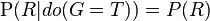 . . If, moreover, we wish to predict the impact of turning the sprinkler on, we have  with the term  removed, showing that the action has an effect on the grass but not on the rain. removed, showing that the action has an effect on the grass but not on the rain. These predictions may not be feasible when some of the variables are unobserved, as in most policy evaluation problems. The effect of the action  can still be predicted, however, whenever a criterion called "back-door" is satisfied.[1] It states that, if a set Z of nodes can be observed that d-separates (or blocks) all back-door paths from X to Y then can still be predicted, however, whenever a criterion called "back-door" is satisfied.[1] It states that, if a set Z of nodes can be observed that d-separates (or blocks) all back-door paths from X to Y then  . A back-door path is one that ends with an arrow into X. Sets that satisfy the back-door criterion are called "sufficient" or "admissible." For example, the set Z = R is admissible for predicting the effect of S = T on G, because R d-separate the (only) back-door path S ← R → G. However, if S is not observed, there is no other set that d-separates this path and the effect of turning the sprinkler on (S = T) on the grass (G) cannot be predicted from passive observations. We then say that P(G|do(S = T)) is not "identified." This reflects the fact that, lacking interventional data, we cannot determine if the observed dependence between S and G is due to a causal connection or is spurious (apparent dependence arising from a common cause, R). (see Simpson's paradox) . A back-door path is one that ends with an arrow into X. Sets that satisfy the back-door criterion are called "sufficient" or "admissible." For example, the set Z = R is admissible for predicting the effect of S = T on G, because R d-separate the (only) back-door path S ← R → G. However, if S is not observed, there is no other set that d-separates this path and the effect of turning the sprinkler on (S = T) on the grass (G) cannot be predicted from passive observations. We then say that P(G|do(S = T)) is not "identified." This reflects the fact that, lacking interventional data, we cannot determine if the observed dependence between S and G is due to a causal connection or is spurious (apparent dependence arising from a common cause, R). (see Simpson's paradox) To determine whether a causal relation is identified from an arbitrary Bayesian network with unobserved variables, one can use the three rules of "do-calculus"[1][2] and test whether all doterms can be removed from the expression of that relation, thus confirming that the desired quantity is estimable from frequency data.[3] Using a Bayesian network can save considerable amounts of memory, if the dependencies in the joint distribution are sparse. For example, a naive way of storing the conditional probabilities of 10 two-valued variables as a table requires storage space for  values. If the local distributions of no variable depends on more than 3 parent variables, the Bayesian network representation only needs to store at most values. If the local distributions of no variable depends on more than 3 parent variables, the Bayesian network representation only needs to store at most  values. values. One advantage of Bayesian networks is that it is intuitively easier for a human to understand (a sparse set of) direct dependencies and local distributions than complete joint distribution. Inference and learning[edit]There are three main inference tasks for Bayesian networks. Inferring unobserved variables[edit]Because a Bayesian network is a complete model for the variables and their relationships, it can be used to answer probabilistic queries about them. For example, the network can be used to find out updated knowledge of the state of a subset of variables when other variables (the evidence variables) are observed. This process of computing the posterior distribution of variables given evidence is called probabilistic inference. The posterior gives a universal sufficient statistic for detection applications, when one wants to choose values for the variable subset which minimize some expected loss function, for instance the probability of decision error. A Bayesian network can thus be considered a mechanism for automatically applyingBayes' theorem to complex problems. The most common exact inference methods are: variable elimination, which eliminates (by integration or summation) the non-observed non-query variables one by one by distributing the sum over the product; clique tree propagation, which caches the computation so that many variables can be queried at one time and new evidence can be propagated quickly; andrecursive conditioning and AND/OR search, which allow for a space-time tradeoff and match the efficiency of variable elimination when enough space is used. All of these methods have complexity that is exponential in the network's treewidth. The most common approximate inference algorithms are importance sampling, stochastic MCMC simulation, mini-bucket elimination, loopy belief propagation, generalized belief propagation, and variational methods. Parameter learning[edit]In order to fully specify the Bayesian network and thus fully represent the joint probability distribution, it is necessary to specify for each node X the probability distribution for Xconditional upon X's parents. The distribution of X conditional upon its parents may have any form. It is common to work with discrete or Gaussian distributions since that simplifies calculations. Sometimes only constraints on a distribution are known; one can then use the principle of maximum entropy to determine a single distribution, the one with the greatestentropy given the constraints. (Analogously, in the specific context of a dynamic Bayesian network, one commonly specifies the conditional distribution for the hidden state's temporal evolution to maximize the entropy rate of the implied stochastic process.) Often these conditional distributions include parameters which are unknown and must be estimated from data, sometimes using the maximum likelihood approach. Direct maximization of the likelihood (or of the posterior probability) is often complex when there are unobserved variables. A classical approach to this problem is the expectation-maximization algorithmwhich alternates computing expected values of the unobserved variables conditional on observed data, with maximizing the complete likelihood (or posterior) assuming that previously computed expected values are correct. Under mild regularity conditions this process converges on maximum likelihood (or maximum posterior) values for parameters. A more fully Bayesian approach to parameters is to treat parameters as additional unobserved variables and to compute a full posterior distribution over all nodes conditional upon observed data, then to integrate out the parameters. This approach can be expensive and lead to large dimension models, so in practice classical parameter-setting approaches are more common. Structure learning[edit]In the simplest case, a Bayesian network is specified by an expert and is then used to perform inference. In other applications the task of defining the network is too complex for humans. In this case the network structure and the parameters of the local distributions must be learned from data. Automatically learning the graph structure of a Bayesian network is a challenge pursued within machine learning. The basic idea goes back to a recovery algorithm developed by Rebane and Pearl (1987)[4] and rests on the distinction between the three possible types of adjacent triplets allowed in a directed acyclic graph (DAG): 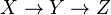 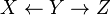 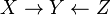 Type 1 and type 2 represent the same dependencies ( and and  are independent given are independent given  ) and are, therefore, indistinguishable. Type 3, however, can be uniquely identified, since and are marginally independent and all other pairs are dependent. Thus, while the skeletons (the graphs stripped of arrows) of these three triplets are identical, the directionality of the arrows is partially identifiable. The same distinction applies when and have common parents, except that one must first condition on those parents. Algorithms have been developed to systematically determine the skeleton of the underlying graph and, then, orient all arrows whose directionality is dictated by the conditional independencies observed.[1][5][6][7] ) and are, therefore, indistinguishable. Type 3, however, can be uniquely identified, since and are marginally independent and all other pairs are dependent. Thus, while the skeletons (the graphs stripped of arrows) of these three triplets are identical, the directionality of the arrows is partially identifiable. The same distinction applies when and have common parents, except that one must first condition on those parents. Algorithms have been developed to systematically determine the skeleton of the underlying graph and, then, orient all arrows whose directionality is dictated by the conditional independencies observed.[1][5][6][7] An alternative method of structural learning uses optimization based search. It requires a scoring function and a search strategy. A common scoring function is posterior probability of the structure given the training data. The time requirement of an exhaustive search returning a structure that maximizes the score is superexponential in the number of variables. A local search strategy makes incremental changes aimed at improving the score of the structure. A global search algorithm like Markov chain Monte Carlo can avoid getting trapped in local minima. Friedman et al.[8][9] talk about using mutual information between variables and finding a structure that maximizes this. They do this by restricting the parent candidate set to knodes and exhaustively searching therein. Statistical introduction[edit]Given data  and parameter and parameter  , a simple Bayesian analysis starts with a prior probability (prior) , a simple Bayesian analysis starts with a prior probability (prior)  and likelihood and likelihood  to compute a posterior probability to compute a posterior probability 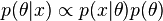 . . Often the prior on depends in turn on other parameters  that are not mentioned in the likelihood. So, the prior must be replaced by a likelihood that are not mentioned in the likelihood. So, the prior must be replaced by a likelihood  , and a prior , and a prior  on the newly introduced parameters is required, resulting in a posterior probability on the newly introduced parameters is required, resulting in a posterior probability  This is the simplest example of a hierarchical Bayes model.[clarification needed]]] The process may be repeated; for example, the parameters may depend in turn on additional parameters  , which will require their own prior. Eventually the process must terminate, with priors that do not depend on any other unmentioned parameters. , which will require their own prior. Eventually the process must terminate, with priors that do not depend on any other unmentioned parameters. Introductory examples[edit] ![[icon]](http://upload.wikimedia.org/wikipedia/commons/thumb/1/1c/Wiki_letter_w_cropped.svg/20px-Wiki_letter_w_cropped.svg.png) | This section requires expansion. (March 2009) | Suppose we have measured the quantities  each with normally distributed errors of known standard deviation each with normally distributed errors of known standard deviation  , , 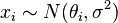 Suppose we are interested in estimating the  . An approach would be to estimate the using a maximum likelihood approach; since the observations are independent, the likelihood factorizes and the maximum likelihood estimate is simply . An approach would be to estimate the using a maximum likelihood approach; since the observations are independent, the likelihood factorizes and the maximum likelihood estimate is simply  However, if the quantities are related, so that for example we may think that the individual have themselves been drawn from an underlying distribution, then this relationship destroys the independence and suggests a more complex model, e.g., 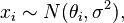  with improper priors  flat, flat,  flat flat . When . When  , this is an identified model (i.e. there exists a unique solution for the model's parameters), and the posterior distributions of the individual will tend to move, or shrink away from the maximum likelihood estimates towards their common mean. This shrinkage is a typical behavior in hierarchical Bayes models. , this is an identified model (i.e. there exists a unique solution for the model's parameters), and the posterior distributions of the individual will tend to move, or shrink away from the maximum likelihood estimates towards their common mean. This shrinkage is a typical behavior in hierarchical Bayes models. Restrictions on priors[edit]Some care is needed when choosing priors in a hierarchical model, particularly on scale variables at higher levels of the hierarchy such as the variable  in the example. The usual priors such as the Jeffreys prior often do not work, because the posterior distribution will be improper (not normalizable), and estimates made by minimizing the expected loss will beinadmissible. in the example. The usual priors such as the Jeffreys prior often do not work, because the posterior distribution will be improper (not normalizable), and estimates made by minimizing the expected loss will beinadmissible. Definitions and concepts[edit]There are several equivalent definitions of a Bayesian network. For all the following, let G = (V,E) be a directed acyclic graph (or DAG), and let X = (Xv)v ∈ V be a set of random variablesindexed by V. Factorization definition[edit]X is a Bayesian network with respect to G if its joint probability density function (with respect to a product measure) can be written as a product of the individual density functions, conditional on their parent variables: 
where pa(v) is the set of parents of v (i.e. those vertices pointing directly to v via a single edge). For any set of random variables, the probability of any member of a joint distribution can be calculated from conditional probabilities using the chain rule (given a topological ordering of X) as follows: 
Compare this with the definition above, which can be written as: 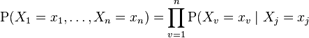 for each for each  which is a parent of which is a parent of 
The difference between the two expressions is the conditional independence of the variables from any of their non-descendents, given the values of their parent variables. Local Markov property[edit]X is a Bayesian network with respect to G if it satisfies the local Markov property: each variable is conditionally independent of its non-descendants given its parent variables:  where de(v) is the set of descendants of v. This can also be expressed in terms similar to the first definition, as 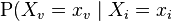 for each for each  which is not a descendent of which is not a descendent of  for each which is a parent of for each which is a parent of Note that the set of parents is a subset of the set of non-descendants because the graph is acyclic. Developing Bayesian networks[edit]To develop a Bayesian network, we often first develop a DAG G such that we believe X satisfies the local Markov property with respect to G. Sometimes this is done by creating a causal DAG. We then ascertain the conditional probability distributions of each variable given its parents in G. In many cases, in particular in the case where the variables are discrete, if we define the joint distribution of X to be the product of these conditional distributions, then X is a Bayesian network with respect to G.[12] Markov blanket[edit]The Markov blanket of a node is the set of nodes consisting of its parents, its children, and any other parents of its children. This set renders it independent of the rest of the network; the joint distribution of the variables in the Markov blanket of a node is sufficient knowledge for calculating the distribution of the node. X is a Bayesian network with respect to G if every node is conditionally independent of all other nodes in the network, given its Markov blanket. d-separation[edit]This definition can be made more general by defining the "d"-separation of two nodes, where d stands for directional.[13][14] Let P be a trail (that is, a collection of edges which is like a path, but each of whose edges may have any direction) from node u to v. Then P is said to be d-separated by a set of nodes Z if and only if (at least) one of the following holds: - P contains a chain, x ← m ← y, such that the middle node m is in Z,
- P contains a fork, x ← m → y, such that the middle node m is in Z, or
- P contains an inverted fork (or collider), x → m ← y, such that the middle node m is not in Z and no descendant of m is in Z.
Thus u and v are said to be d-separated by Z if all trails between them are d-separated. If u and v are not d-separated, they are called d-connected. X is a Bayesian network with respect to G if, for any two nodes u, v: 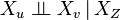 where Z is a set which d-separates u and v. (The Markov blanket is the minimal set of nodes which d-separates node v from all other nodes.) Hierarchical models[edit]The term hierarchical model is sometimes considered a particular type of Bayesian network, but has no formal definition. Sometimes the term is reserved for models with three or more levels of random variables; other times, it is reserved for models with latent variables. In general, however, any moderately complex Bayesian network is usually termed "hierarchical". Causal networks[edit]Although Bayesian networks are often used to represent causal relationships, this need not be the case: a directed edge from u to v does not require that Xv is causally dependent onXu. This is demonstrated by the fact that Bayesian networks on the graphs:  are equivalent: that is they impose exactly the same conditional independence requirements. A causal network is a Bayesian network with an explicit requirement that the relationships be causal. The additional semantics of the causal networks specify that if a node X is actively caused to be in a given state x (an action written as do(X=x)), then the probability density function changes to the one of the network obtained by cutting the links from X's parents to X, and setting X to the caused value x.[1] Using these semantics, one can predict the impact of external interventions from data obtained prior to intervention. Applications[edit]Bayesian networks are used for modelling knowledge in computational biology and bioinformatics (gene regulatory networks, protein structure, gene expression analysis,[15] learning epistasis from GWAS data sets [16]) medicine,[17] biomonitoring,[18] document classification, information retrieval,[19] semantic search,[20] image processing, data fusion, decision support systems,[21] engineering, gaming and law.[22][23][24] Software[edit] - WinBUGS
- OpenBUGS (website), further (open source) development of WinBUGS.
- OpenMarkov, open source software and API implemented in Java
- Just another Gibbs sampler (JAGS) (website)
- Stan (website) — Stan is an open-source package for obtaining Bayesian inference using the No-U-Turn sampler, a variant of Hamiltonian Monte Carlo. It’s somewhat like BUGS, but with a different language for expressing models and a different sampler for sampling from their posteriors. RStan is the R interface to Stan.
- GeNIe&Smile (website) — SMILE is a C++ library for BN and ID, and GeNIe is a GUI for it
- SamIam (website), a Java-based system with GUI and Java API
- Bayes Server - User Interface and API for Bayesian networks, includes support for time series and sequences
- Belief and Decision Networks on AIspace
- BayesiaLab by Bayesia
- Hugin
- Netica by Norsys
- dVelox by Apara Software
- System Modeler by Inatas AB
History[edit]The term "Bayesian networks" was coined by Judea Pearl in 1985 to emphasize three aspects:[25] - The often subjective nature of the input information.
- The reliance on Bayes' conditioning as the basis for updating information.
- The distinction between causal and evidential modes of reasoning, which underscores Thomas Bayes' posthumously published paper of 1763.[26]
In the late 1980s the seminal texts Probabilistic Reasoning in Intelligent Systems[27] and Probabilistic Reasoning in Expert Systems[28] summarized the properties of Bayesian networks and helped to establish Bayesian networks as a field of study. Informal variants of such networks were first used by legal scholar John Henry Wigmore, in the form of Wigmore charts, to analyse trial evidence in 1913.[23]:66–76 Another variant, calledpath diagrams, was developed by the geneticist Sewall Wright[29] and used in social and behavioral sciences (mostly with linear parametric models). - ^ Jump up to:a b c d Pearl, Judea (2000). Causality: Models, Reasoning, and Inference. Cambridge University Press. ISBN 0-521-77362-8.
- Jump up^ J., Pearl (1994). "A Probabilistic Calculus of Actions". In Lopez de Mantaras, R.; Poole, D. UAI'94 Proceedings of the Tenth international conference on Uncertainty in artificial intelligence. San Mateo CA: Morgan Kaufman. pp. 454–462. ISBN 1-55860-332-8.
- Jump up^ I. Shpitser, J. Pearl, "Identification of Conditional Interventional Distributions" In R. Dechter and T.S. Richardson (Eds.), Proceedings of the Twenty-Second Conference on Uncertainty in Artificial Intelligence, 437–444, Corvallis, OR: AUAI Press, 2006.
- Jump up^ Rebane, G. and Pearl, J., "The Recovery of Causal Poly-trees from Statistical Data,"Proceedings, 3rd Workshop on Uncertainty in AI, (Seattle, WA) pages 222–228, 1987
- Jump up^ Spirtes, P.; Glymour, C. (1991). "An algorithm for fast recovery of sparse causal graphs" (PDF). Social Science Computer Review 9 (1): 62–72.doi:10.1177/089443939100900106.
- Jump up^ Spirtes, Peter; Glymour, Clark N.; Scheines, Richard (1993). Causation, Prediction, and Search (1st ed.). Springer-Verlag. ISBN 978-0-387-97979-3.
- Jump up^ Verma, Thomas; Pearl, Judea (1991). "Equivalence and synthesis of causal models". In Bonissone, P.; Henrion, M.; Kanal, L.N. et al. UAI '90 Proceedings of the Sixth Annual Conference on Uncertainty in Artificial Intelligence. Elsevier. pp. 255–270. ISBN 0-444-89264-8.
- Jump up^ Friedman, N.; Geiger, D.; Goldszmidt, M. (1997). Machine Learning 29 (2/3): 131.doi:10.1023/A:1007465528199. edit
- Jump up^ Friedman, N.; Linial, M.; Nachman, I.; Pe'er, D. (2000). "Using Bayesian Networks to Analyze Expression Data". Journal of Computational Biology 7 (3–4): 601–620.doi:10.1089/106652700750050961. PMID 11108481. edit
- Jump up^ Neapolitan, Richard E. (2004). Learning Bayesian networks. Prentice Hall. ISBN 978-0-13-012534-7.
- Jump up^ Geiger, Dan; Verma, Thomas; Pearl, Judea (1990). "Identifying independence in Bayesian Networks" (PDF). Networks 20: 507–534.doi:10.1177/089443939100900106.
- Jump up^ Richard Scheines, D-separation
- Jump up^ N. Friedman, M. Linial, I. Nachman, D. Pe'er (August 2000). "Using Bayesian Networks to Analyze Expression Data". Journal of Computational Biology (Larchmont, New York:Mary Ann Liebert, Inc.) 7 (3/4): 601–620. doi:10.1089/106652700750050961.ISSN 1066-5277. PMID 11108481.
- Jump up^ Jiang, X.; Neapolitan, R.E.; Barmada, M.M.; Visweswaran, S. (2011). "Learning Genetic Epistasis using Bayesian Network Scoring Criteria". BMC Bioinformatics 12: 89.doi:10.1186/1471-2105-12-89. PMC 3080825. PMID 21453508.
- Jump up^ J. Uebersax (2004). Genetic Counseling and Cancer Risk Modeling: An Application of Bayes Nets. Marbella, Spain: Ravenpack International.
- Jump up^ Jiang X, Cooper GF. (July–August 2010). "A Bayesian spatio-temporal method for disease outbreak detection". J Am Med Inform Assoc 17 (4): 462–71.doi:10.1136/jamia.2009.000356. PMC 2995651. PMID 20595315.
- Jump up^ Luis M. de Campos, Juan M. Fernández-Luna and Juan F. Huete (2004). "Bayesian networks and information retrieval: an introduction to the special issue". Information Processing & Management (Elsevier) 40 (5): 727–733. doi:10.1016/j.ipm.2004.03.001.ISBN 0-471-14182-8.
- Jump up^ Christos L. Koumenides and Nigel R. Shadbolt. 2012. Combining link and content-based information in a Bayesian inference model for entity search. In Proceedings of the 1st Joint International Workshop on Entity-Oriented and Semantic Search (JIWES '12). ACM, New York, NY, USA, , Article 3 , 6 pages. DOI=10.1145/2379307.2379310
- Jump up^ F.J. Díez, J. Mira, E. Iturralde and S. Zubillaga (1997). "DIAVAL, a Bayesian expert system for echocardiography". Artificial Intelligence in Medicine (Elsevier) 10 (1): 59–73.PMID 9177816.
- Jump up^ G. A. Davis (2003). "Bayesian reconstruction of traffic accidents". Law, Probability and Risk 2 (2): 69–89. doi:10.1093/lpr/2.2.69.
- ^ Jump up to:a b J. B. Kadane and D. A. Schum (1996). A Probabilistic Analysis of the Sacco and Vanzetti Evidence. New York: Wiley. ISBN 0-471-14182-8.
- Jump up^ O. Pourret, P. Naim and B. Marcot (2008). Bayesian Networks: A Practical Guide to Applications. Chichester, UK: Wiley. ISBN 978-0-470-06030-8.
- Jump up^ Pearl, J. (1985). "Bayesian Networks: A Model of Self-Activated Memory for Evidential Reasoning" (UCLA Technical Report CSD-850017). Proceedings of the 7th Conference of the Cognitive Science Society, University of California, Irvine, CA. pp. 329–334. Retrieved 2009-05-01.
- Jump up^ Bayes, T.; Price, Mr. (1763). "An Essay towards solving a Problem in the Doctrine of Chances". Philosophical Transactions of the Royal Society of London 53: 370–418.doi:10.1098/rstl.1763.0053.
- Jump up^ Pearl, J. Probabilistic Reasoning in Intelligent Systems. San Francisco CA: Morgan Kaufmann. p. 1988. ISBN 1558604790.
- Jump up^ Neapolitan, Richard E. (1989). Probabilistic reasoning in expert systems: theory and algorithms. Wiley. ISBN 978-0-471-61840-9.
- Jump up^ Wright, S. (1921). "Correlation and Causation" (PDF). Journal of Agricultural Research 20 (7): 557–585.
General references[edit] - Ben-Gal, Irad (2007). Bayesian Networks (PDF). In Ruggeri, Fabrizio; Kennett, Ron S.; Faltin, Frederick W. "Encyclopedia of Statistics in Quality and Reliability". Encyclopedia of Statistics in Quality and Reliability. John Wiley & Sons.doi:10.1002/9780470061572.eqr089. ISBN 978-0-470-01861-3.
- Bertsch McGrayne, Sharon. The Theory That Would not Die. Yale.
- Borgelt, Christian; Kruse, Rudolf (March 2002). Graphical Models: Methods for Data Analysis and Mining. Chichester, UK: Wiley. ISBN 0-470-84337-3.
- Borsuk, Mark Edward (2008). "Ecological informatics: Bayesian networks". In Jørgensen , Sven Erik, Fath, Brian. Encyclopedia of Ecology. Elsevier. ISBN 978-0-444-52033-3.
- Castillo, Enrique; Gutiérrez, José Manuel; Hadi, Ali S. (1997). "Learning Bayesian Networks".Expert Systems and Probabilistic Network Models. Monographs in computer science. New York: Springer-Verlag. pp. 481–528. ISBN 0-387-94858-9.
- Comley, Joshua W.; Dowe, David L. (October 2003). "Minimum Message Length and Generalized Bayesian Nets with Asymmetric Languages". Written at Victoria, Australia. In Grünwald, Peter D.; Myung, In Jae; Pitt, Mark A. Advances in Minimum Description Length: Theory and Applications. Neural information processing series. Cambridge, Massachusetts: Bradford Books (MIT Press) (published April 2005). pp. 265–294. ISBN 0-262-07262-9. (This paper puts decision trees in internal nodes of Bayes networks using Minimum Message Length (MML). An earlier version is Comley and Dowe (2003), .pdf.)
- Darwiche, Adnan (2009). Modeling and Reasoning with Bayesian Networks. Cambridge University Press. ISBN 978-0521884389.
- Dowe, David L. (2010). MML, hybrid Bayesian network graphical models, statistical consistency, invariance and uniqueness, in Handbook of Philosophy of Science (Volume 7: Handbook of Philosophy of Statistics), Elsevier, ISBN 978-0-444-51862-0, pp 901–982.
- Fenton, Norman; Neil, Martin E. (November 2007). Managing Risk in the Modern World: Applications of Bayesian Networks – A Knowledge Transfer Report from the London Mathematical Society and the Knowledge Transfer Network for Industrial Mathematics.London (England): London Mathematical Society.
- Fenton, Norman; Neil, Martin E. (July 23, 2004). "Combining evidence in risk analysis using Bayesian Networks" (PDF). Safety Critical Systems Club Newsletter 13 (4) (Newcastle upon Tyne, England). pp. 8–13.
- Andrew Gelman; John B Carlin; Hal S Stern; Donald B Rubin (2003). "Part II: Fundamentals of Bayesian Data Analysis: Ch.5 Hierarchical models". Bayesian Data Analysis. CRC Press. pp. 120–. ISBN 978-1-58488-388-3.
- Heckerman, David (March 1, 1995). "Tutorial on Learning with Bayesian Networks". In Jordan, Michael Irwin. Learning in Graphical Models. Adaptive Computation and Machine Learning. Cambridge, Massachusetts: MIT Press (published 1998). pp. 301–354. ISBN 0-262-60032-3..
- Also appears as Heckerman, David (March 1997). "Bayesian Networks for Data Mining". Data Mining and Knowledge Discovery (Netherlands: Springer Netherlands) 1 (1): 79–119.doi:10.1023/A:1009730122752. ISSN 1384-5810.
- An earlier version appears as Technical Report MSR-TR-95-06, Microsoft Research, March 1, 1995. The paper is about both parameter and structure learning in Bayesian networks.
- Jensen, Finn V; Nielsen, Thomas D. (June 6, 2007). Bayesian Networks and Decision Graphs. Information Science and Statistics series (2nd ed.). New York: Springer-Verlag.ISBN 978-0-387-68281-5.
- Korb, Kevin B.; Nicholson, Ann E. (December 2010). Bayesian Artificial Intelligence. CRC Computer Science & Data Analysis (2nd ed.). Chapman & Hall (CRC Press).doi:10.1007/s10044-004-0214-5. ISBN 1-58488-387-1.
- Lunn, D.; et al., D; Thomas, A; Best, N (2009). "The BUGS project: Evolution, critique and future directions". Statistics in Medicine 28 (25): 3049–3067. doi:10.1002/sim.3680.PMID 19630097.
- Neil, Martin; Fenton, Norman E.; Tailor, Manesh (August 2005). "Using Bayesian Networks to Model Expected and Unexpected Operational Losses" (pdf). In Greenberg, Michael R. Risk Analysis: an International Journal (John Wiley & Sons) 25 (4): 963–972. doi:10.1111/j.1539-6924.2005.00641.x. PMID 16268944.
- Pearl, Judea (September 1986). "Fusion, propagation, and structuring in belief networks".Artificial Intelligence (Elsevier) 29 (3): 241–288. doi:10.1016/0004-3702(86)90072-X.ISSN 0004-3702.
- Pearl, Judea (1988). Probabilistic Reasoning in Intelligent Systems: Networks of Plausible Inference. Representation and Reasoning Series (2nd printing ed.). San Francisco, California: Morgan Kaufmann. ISBN 0-934613-73-7.
- Pearl, Judea; Russell, Stuart (November 2002). "Bayesian Networks". In Arbib, Michael A..Handbook of Brain Theory and Neural Networks. Cambridge, Massachusetts: Bradford Books (MIT Press). pp. 157–160. ISBN 0-262-01197-2.
- Russell, Stuart J.; Norvig, Peter (2003), Artificial Intelligence: A Modern Approach (2nd ed.), Upper Saddle River, New Jersey: Prentice Hall, ISBN 0-13-790395-2.
- Zhang, Nevin Lianwen; Poole, David (May 1994). "A simple approach to Bayesian network computations". Proceedings of the Tenth Biennial Canadian Artificial Intelligence Conference (AI-94). (Banff, Alberta): 171–178. This paper presents variable elimination for belief networks.
- Computational Intelligence: A Methodological Introduction by Kruse, Borgelt, Klawonn, Moewes, Steinbrecher, Held, 2013, Springer, ISBN 9781447150121
- Graphical Models - Representations for Learning, Reasoning and Data Mining, 2nd Edition, by Borgelt, Steinbrecher, Kruse, 2009, J. Wiley & Sons, ISBN 9780470749562
External links[edit] |
+Citations (1) - CitationsAdd new citationList by: CiterankMapLink[1] Wikipedia
Author: Various
Cited by: Roger Yau 5:15 PM 19 October 2013 GMT
Citerank: (28) 291862AODE - Averaged one-dependence estimatorsAveraged one-dependence estimators (AODE) is a probabilistic classification learning technique. It was developed to address the attribute-independence problem of the popular naive Bayes classifier. It frequently develops substantially more accurate classifiers than naive Bayes at the cost of a modest increase in the amount of computation.109FDEF6, 291863Artificial neural networkIn computer science and related fields, artificial neural networks are computational models inspired by animal central nervous systems (in particular the brain) that are capable of machine learning and pattern recognition. They are usually presented as systems of interconnected "neurons" that can compute values from inputs by feeding information through the network.109FDEF6, 291936BackpropagationBackpropagation, an abbreviation for "backward propagation of errors", is a common method of training artificial neural networks. From a desired output, the network learns from many inputs, similar to the way a child learns to identify a dog from examples of dogs.109FDEF6, 291937Bayesian statisticsBayesian statistics is a subset of the field of statistics in which the evidence about the true state of the world is expressed in terms of degrees of belief or, more specifically, Bayesian probabilities. Such an interpretation is only one of a number of interpretations of probability and there are other statistical techniques that are not based on "degrees of belief".109FDEF6, 291938Naive Bayes classifierA naive Bayes classifier is a simple probabilistic classifier based on applying Bayes' theorem with strong (naive) independence assumptions. A more descriptive term for the underlying probability model would be "independent feature model". An overview of statistical classifiers is given in the article on Pattern recognition.109FDEF6, 291941Case-based reasoningCase-based reasoning (CBR), broadly construed, is the process of solving new problems based on the solutions of similar past problems. An auto mechanic who fixes an engine by recalling another car that exhibited similar symptoms is using case-based reasoning. So, too, an engineer copying working elements of nature (practicing biomimicry), is treating nature as a database of solutions to problems. Case-based reasoning is a prominent kind of analogy making.109FDEF6, 291942Decision tree learningDecision tree learning uses a decision tree as a predictive model which maps observations about an item to conclusions about the item's target value. It is one of the predictive modelling approaches used in statistics, data mining and machine learning. More descriptive names for such tree models are classification trees or regression trees. In these tree structures, leaves represent class labels and branches represent conjunctions of features that lead to those class labels.109FDEF6, 291943Inductive logic programmingInductive logic programming (ILP) is a subfield of machine learning which uses logic programming as a uniform representation for examples, background knowledge and hypotheses. Given an encoding of the known background knowledge and a set of examples represented as a logical database of facts, an ILP system will derive a hypothesised logic program which entails all the positive and none of the negative examples.109FDEF6, 291944Gaussian process regression (Kriging)Kriging is a method to build an approximation of a function from a set of evaluations of the function at a finite set of points. The method originates from the domain of geostatistics and is now widely used in the domain of spatial analysis and computer experiments. The technique is also known as Gaussian process regression, Kolmogorov Wiener prediction, or Best Linear Unbiased Prediction.109FDEF6, 291945Gene expression programmingGene expression programming (GEP) is an evolutionary algorithm that creates computer programs or models. These computer programs are complex tree structures that learn and adapt by changing their sizes, shapes, and composition, much like a living organism. And like living organisms, the computer programs of GEP are also encoded in simple linear chromosomes of fixed length. Thus, GEP is a genotype-phenotype system.109FDEF6, 291946Group method of data handlingGroup method of data handling (GMDH) is a family of inductive algorithms for computer-based mathematical modeling of multi-parametric datasets that features fully automatic structural and parametric optimization of models.109FDEF6, 291947Learning automataA branch of the theory of adaptive control is devoted to learning automata surveyed by Narendra and Thathachar which were originally described explicitly as finite state automata. Learning automata select their current action based on past experiences from the environment.109FDEF6, 291948Supervised learningSupervised learning is the machine learning task of inferring a function from labeled training data.[1] The training data consist of a set of training examples. In supervised learning, each example is a pair consisting of an input object (typically a vector) and a desired output value (also called the supervisory signal). A supervised learning algorithm analyzes the training data and produces an inferred function, which can be used for mapping new examples. 25CBCBFF, 291950Unsupervised learningIn machine learning, the problem of unsupervised learning is that of trying to find hidden structure in unlabeled data. Since the examples given to the learner are unlabeled, there is no error or reward signal to evaluate a potential solution. This distinguishes unsupervised learning from supervised learning and reinforcement learning.25CBCBFF, 291951Reinforcement learningReinforcement learning is an area of machine learning inspired by behaviorist psychology, concerned with how software agents ought to take actions in an environment so as to maximize some notion of cumulative reward. The problem, due to its generality, is studied in many other disciplines, such as game theory, control theory, operations research, information theory, simulation-based optimization, statistics, and genetic algorithms.25CBCBFF, 292450Hierarchical clusteringIn data mining, hierarchical clustering is a method of cluster analysis which seeks to build a hierarchy of clusters. Strategies for hierarchical clustering generally fall into two types:
Agglomerative: This is a "bottom up" approach: each observation starts in its own cluster, and pairs of clusters are merged as one moves up the hierarchy.
Divisive: This is a "top down" approach: all observations start in one cluster, and splits are performed recursively as one moves down the hierarch109FDEF6, 292451Association rule learningAssociation rule learning is a popular and well researched method for discovering interesting relations between variables in large databases. It is intended to identify strong rules discovered in databases using different measures of interestingness.109FDEF6, 292454Others25CBCBFF, 292455Learning Vector QuantizationIn computer science, Learning Vector Quantization (LVQ), is a prototype-based supervised classification algorithm. LVQ is the supervised counterpart of vector quantization systems.
LVQ can be understood as a special case of an artificial neural network, more precisely, it applies a winner-take-all Hebbian learning-based approach. It is a precursor to Self-organizing maps (SOM) and related to Neural gas, and to the k-Nearest Neighbor algorithm (k-NN). LVQ was invented by Teuvo Kohonen.109FDEF6, 292463Logistic Model TreeLMT is a classification model with an associated supervised training algorithm that combines logistic regression (LR) and decision tree learning. Logistic model trees are based on the earlier idea of a model tree: a decision tree that has linear regression models at its leaves to provide a piecewise linear regression model (where ordinary decision trees with constants at their leaves would produce a piecewise constant model).109FDEF6, 292464Minimum message lengthMinimum message length (MML) is a formal information theory restatement of Occam's Razor: even when models are not equal in goodness of fit accuracy to the observed data, the one generating the shortest overall message is more likely to be correct (where the message consists of a statement of the model, followed by a statement of data encoded concisely using that model). MML was invented by Chris Wallace, first appearing in the seminal (Wallace and Boulton, 1968).109FDEF6, 292465Lazy learningIn artificial intelligence, lazy learning is a learning method in which generalization beyond the training data is delayed until a query is made to the system, as opposed to in eager learning, where the system tries to generalize the training data before receiving queries.109FDEF6, 292466Instance-based learninginstance-based learning or memory-based learning is a family of learning algorithms that, instead of performing explicit generalization, compare new problem instances with instances seen in training, which have been stored in memory. Instance-based learning is a kind of lazy learning.109FDEF6, 292475k-nearest neighbor algorithmIn pattern recognition, the k-nearest neighbor algorithm (k-NN) is a non-parametric method for classifying objects based on closest training examples in the feature space. k-NN is a type of instance-based learning, or lazy learning where the function is only approximated locally and all computation is deferred until classification. 109FDEF6, 292476Analogical modelingAnalogical modeling (hereafter AM) is a formal theory of exemplar-based analogical reasoning, proposed by Royal Skousen, professor of Linguistics and English language at Brigham Young University in Provo, Utah. It is applicable to language modeling and other categorization tasks. Analogical modeling is related to connectionism and nearest neighbor approaches, in that it is data-based rather than abstraction-based.109FDEF6, 292478Probably approximately correct learningIn this framework, the learner receives samples and must select a generalization function (called the hypothesis) from a certain class of possible functions. The goal is that, with high probability (the "probably" part), the selected function will have low generalization error (the "approximately correct" part). The learner must be able to learn the concept given any arbitrary approximation ratio, probability of success, or distribution of the samples.109FDEF6, 292480Ripple-down rulesRipple Down Rules is a way of approaching knowledge acquisition. Knowledge acquisition refers to the transfer of knowledge from human experts to knowledge based systems.109FDEF6, 292481Support vector machinesIn machine learning, support vector machines (SVMs, also support vector networks[1]) are supervised learning models with associated learning algorithms that analyze data and recognize patterns, used for classification and regression analysis. 109FDEF6 URL: |
|
|