Backpropagation, an abbreviation for "backward propagation of errors", is a common method of training artificial neural networks. From a desired output, the network learns from many inputs, similar to the way a child learns to identify a dog from examples of dogs.
It is a supervised learning method, and is a generalization of the delta rule. It requires a dataset of the desired output for many inputs, making up the training set. It is most useful for feed-forward networks (networks that have no feedback, or simply, that have no connections that loop). Backpropagation requires that the activation function used by the artificial neurons(or "nodes") be differentiable.
Contents
[hide] - 1 Motivation
- 2 Summary
- 2.1 Phase 1: Propagation
- 2.2 Phase 2: Weight update
- 3 Algorithm
- 4 Intuition
- 4.1 Learning as an optimization problem
- 4.2 An analogy for understanding gradient descent
- 5 Derivation
- 6 Modes of learning
- 7 Multithreaded backpropagation
- 8 Limitations
- 9 History
- 10 Notes
- 11 References
- 12 External links
Motivation[edit]
The goal of any supervised learning algorithm is to find a function that best maps a set of inputs to its correct output. An example would be a simple classification task, where the input is an image of an animal, and the correct output would be the name of the animal. Some input and output patterns can be easily learned by single-layer neural networks (i.e. perceptrons). However, these single-layer perceptrons cannot learn some relatively simple patterns, such as those that are not linearly separable. For example, a human may classify an image of an animal by recognizing certain features such as the number of limbs, the texture of the skin (whether it is furry, feathered, scaled, etc.), the size of the animal, and the list goes on. A single-layer neural network however, must learn a function that outputs a label solely using the intensity of the pixels in the image. There is no way for it to learn any abstract features of the input since it is limited to having only one layer. A multi-layered network overcomes this limitation as it can create internal representations and learn different features in each layer.[1]The first layer may be responsible for learning the orientations of lines using the inputs from the individual pixels in the image. The second layer may combine the features learned in the first layer and learn to identify simple shapes such as circles. Each higher layer learns more and more abstract features such as those mentioned above that can be used to classify the image. Each layer finds patterns in the layer below it and it is this ability to create internal representations that are independent of outside input that gives multi-layered networks its power. The goal and motivation for developing the backpropagation algorithm is to find a way to train multi-layered neural networks such that it can learn the appropriate internal representations to allow it to learn any arbitrary mapping of input to output.[1]
Summary[edit]
For better understanding, the backpropagation learning algorithm can be divided into two phases: propagation and weight update.
Phase 1: Propagation[edit]
Each propagation involves the following steps:
- Forward propagation of a training pattern's input through the neural network in order to generate the propagation's output activations.
- Backward propagation of the propagation's output activations through the neural network using the training pattern target in order to generate the deltas of all output and hidden neurons.
Phase 2: Weight update[edit]
For each weight-synapse follow the following steps:
- Multiply its output delta and input activation to get the gradient of the weight.
- Subtract a ratio (percentage) of the gradient from the weight.
This ratio (percentage) influences the speed and quality of learning; it is called the learning rate. The greater the ratio, the faster the neuron trains; the lower the ratio, the more accurate the training is. The sign of the gradient of a weight indicates where the error is increasing, this is why the weight must be updated in the opposite direction.
Repeat phase 1 and 2 until the performance of the network is satisfactory.
Algorithm[edit]
Algorithm for a 3-layer network (only one hidden layer):
initialize network weights (often small random values) do forEach training example ex prediction = neural-net-output(network, ex) // forward pass actual = teacher-output(ex) compute error (prediction - actual) at the output units compute  for all weights from hidden layer to output layer // backward pass compute
  for all weights from input layer to hidden layer // backward pass continued update network weights until all examples classified correctly or stopping criterion satisfied return the network
As the algorithm's name implies, the errors propagate backwards from the output nodes to the input nodes. Technically speaking, backpropagation calculates the gradient of the error of the network regarding the network's modifiable weights.[2] This gradient is almost always used in a simple stochastic gradient descent algorithm to find weights that minimize the error. Often the term "backpropagation" is used in a more general sense, to refer to the entire procedure encompassing both the calculation of the gradient and its use in stochastic gradient descent. Backpropagation usually allows quick convergence on satisfactory local minima for error in the kind of networks to which it is suited.
Backpropagation networks are necessarily multilayer perceptrons (usually with one input, one hidden, and one output layer). In order for the hidden layer to serve any useful function, multilayer networks must have non-linear activation functions for the multiple layers: a multilayer network using only linear activation functions is equivalent to some single layer, linear network. Non-linear activation functions that are commonly used include the logistic function, the softmax function, and the gaussian function.
The backpropagation algorithm for calculating a gradient has been rediscovered a number of times, and is a special case of a more general technique called automatic differentiation in the reverse accumulation mode.
It is also closely related to the Gauss–Newton algorithm, and is also part of continuing research in neural backpropagation.
Intuition[edit]
Learning as an optimization problem[edit]
Before showing the mathematical derivation of the backpropagation algorithm, it helps to develop some intuitions about the relationship between the actual output of a neuron and the correct output for a particular training case. Consider a simple neural network with two input units, one output unit and no hidden units. Each neuron uses a linear output[note 1] that is the weighted sum of its input.

A simple neural network with two input units and one output unit
Initially, before training, the weights will be set randomly. Then the neuron learns from training examples, which in this case consists of a set of tuples ( ,
,  ,
,  ) where and are the inputs to the network and is the correct output (the output the network should eventually produce given the identical inputs). The network given and will compute an output
  which very likely differs from (since the weights are initially random). A common method for measuring the discrepancy between the expected output and the actual output is using the squared error measure:
 ,
,
where  is the discrepancy or error.
As an example, consider the network on a single training case: (1, 1, 0), thus the input and are 1 and 1 respectively and the correct output, is 0. Now if the actual output is plotted on the x-axis against the error on the y-axis, the result is a parabola. Theminima of the parabola corresponds to the output which minimizes the error . For a single training case, the minima also touches the x-axis, which means the error will be zero and the network can produce an output y that exactly matches the expected output . Therefore, the problem of mapping inputs to outputs can be reduced to an optimization problem of finding a function that will produce the minimal error.

Error surface of a linear neuron for a single training case.
However, the output of a neuron depends on the weighted sum of all its inputs:
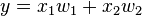 ,
,
where  and
and  are the weights on the connection from the input units to the output unit. Therefore, the error also depends on the incoming weights to the neuron, which is ultimately what needs to be changed in the network to enable learning. If each weight is plotted on a separate horizontal axis and the error on the vertical axis, the result is a parabolic bowl (If a neuron has k weights, then thedimension of the error surface would be k+1, thus a k+1 dimensional equivalent of the 2D parabola).

Error surface of a linear neuron with two input weights
The backpropagation algorithm aims to find the set of weights that minimizes the error. There are several methods for finding the minima of a parabola or any function in any dimension. One way is analytically by solving systems of equations, however this relies on the network being a linear system, and the goal is to be able to also train multi-layer, non-linear networks (since a multi-layered linear network is equivalent to a single-layer network). The method used in backpropagation is gradient descent.
An analogy for understanding gradient descent[edit]
The basic intuition behind gradient descent can be illustrated by a hypothetical scenario. A person is stuck in the mountains is trying to get down (i.e. trying to find the minima). There is heavy fog such that visibility is extremely low. Therefore, the path down the mountain is not visible, so he must use local information to find the minima. He can use the method of gradient descent, which involves looking at the steepness of the hill at his current position, then proceeding in the direction with the most negative steepness (i.e. downhill). If he was trying to find the top of the mountain (i.e. the maxima), then he would proceed in the direction with most positive steepness (i.e. uphill). Using this method, he would eventually find his way down the mountain. However, assume also that the steepness of the hill is not immediately obvious with simple observation, but rather it requires a sophisticated instrument to measure, which the person happens to have at the moment. It takes quite some time to measure the steepness of the hill with the instrument, thus he should minimize his use of the instrument if he wanted to get down the mountain before sunset. The difficulty then is choosing the frequency at which he should measure the steepness of the hill so not to go off track.
In this analogy, the person represents the backpropagation algorithm, and the path down the mountain represents the set of weights that will minimize the error. The steepness of the hill represents the slope of the error surface at that point. The direction he must travel in corresponds to the gradient of the error surface at that point. The instrument used to measure steepness is differentiation (the slope of the error surface can be calculated by taking the derivative of the squared error function at that point). The distance he travels in between measurements (which is also proportional to the frequency as which he takes measurement) is the learning rate of the algorithm. See the limitation section for a discussion of the limitations of this type of "hill climbing" algorithm.
Derivation[edit]
Since backpropagation uses the gradient descent method, one needs to calculate the derivative of the squared error function with respect to the weights of the network. The squared error function is:
| 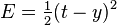 , , |
| = the squared error |
| = target output |
| = actual output of the output neuron[note 2] |
(The  term is added to cancel the exponent when differentiating.) Therefore the error, , depends on the output . However, the output depends on the weighted sum of all its input:
|  |
|  = the number of input units to the neuron = the number of input units to the neuron |
|  = the ith weight = the ith weight |
|  = the ith input value to the neuron = the ith input value to the neuron |
The above formula only holds true for a neuron with a linear activation function (that is the output is solely the weighted sum of the input). In general, a non-linear, differentiable activation function,  , is used. Thus, more correctly:
This lays the groundwork for calculating the partial derivative of the error with respect to a weight using the chain rule:
| 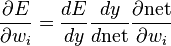 |
|  = How the error changes when the weights are changed = How the error changes when the weights are changed |
|  = How the error changes when the output is changed = How the error changes when the output is changed |
|  = How the output changes when the weighted sum changes = How the output changes when the weighted sum changes |
|  = How the weighted sum changes as the weights change = How the weighted sum changes as the weights change |
Since the weighted sum  is just the sum over all products , therefore the partial derivative of the sum with respect to a weight is the just the corresponding input . Similarly, the partial derivative of the sum with respect to an input value is just the weight :
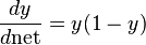
The derivative of the output with respect to the weighted sum is simply the derivative of the activation function :
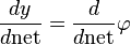
This is the reason why backpropagation requires the activation function to be differentiable. A commonly used activation function is the logistic function:
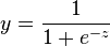
which has a nice derivative of:
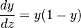
For example purposes, assume the network uses a logistic activation function, in which case the derivative of the output with respect to the weighted sum is the same as the derivative of the logistic function:
Finally, the derivative of the error with respect to the output is:
Putting it all together:
If one were to use a different activation function, the only difference would be the  term will be replaced by the derivative of the newly chosen activation function.
To update the weight using gradient descent, one must choose a learning rate,  . The change in weight after learning then would be the product of the learning rate and the gradient:
For a linear neuron, the derivative of the activation function is 1, which yields:
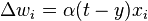
This is exactly the delta rule for perceptron learning, which is why the backpropagation algorithm is a generalization of the delta rule. In backpropagation and perceptron learning, when the output matches the desired output , the change in weight would be zero, which is exactly what is desired.
Modes of learning[edit]
There are three modes of learning to choose from: on-line, batch and stochastic. In on-line and stochastic learning, each propagation is followed immediately by a weight update. In batch learning, many propagations occur before updating the weights. Batch learning requires more memory capacity, but on-line and stochastic learning require more updates. On-line learning is used for dynamic environments that provide a continuous stream of new patterns. Stochastic learning and batch learning both make use of a training set of static patterns. Stochastic goes through the data set in a random order in order to reduce its chances of getting stuck in local minima. Stochastic learning is also much faster than batch learning since weights are updated immediately after each propagation. Yet batch learning will yield a much more stable descent to a local minima since each update is performed based on all patterns.
Multithreaded backpropagation[edit]
Backpropagation is an iterative process that can often take a great deal of time to complete. When multicore computers are used multithreaded techniques can greatly decrease the amount of time that backpropagation takes to converge. If batching is being used, it is relatively simple to adapt the backpropagation algorithm to operate in a multithreaded manner.
The training data is broken up into equally large batches for each of the threads. Each thread executes the forward and backward propagations. The weight and threshold deltas are summed for each of the threads. At the end of each iteration all threads must pause briefly for the weight and threshold deltas to be summed and applied to the neural network. This process continues for each iteration. This multithreaded approach to backpropagation is used by the Encog Neural Network Framework.[3]
Limitations[edit]
- The result may converge to a local minimum. The "hill climbing" strategy of gradient descent is guaranteed to work if there is only one minimum. However, oftentimes the error surface has many local minima and maxima. If the starting point of the gradient descent happens to be somewhere between a local maximum and local minimum, then going down the direction with the most negative gradient will lead to the local minimum.

Gradient descent can find the local minimum instead of the global minimum
- The convergence obtained from backpropagation learning is very slow.
- The convergence in backpropagation learning is not guaranteed.
- Backpropagation learning does not require or normalization of input vectors; however, normalization could improve performance.[4]
History[edit]
Vapnik cites (Bryson, A.E.; W.F. Denham; S.E. Dreyfus. Optimal programming problems with inequality constraints. I: Necessary conditions for extremal solutions. AIAA J. 1, 11 (1963) 2544-2550) as the first publication of the backpropagation algorithm in his book "Support Vector Machines.". Arthur E. Bryson and Yu-Chi Ho described it as a multi-stage dynamic system optimization method in 1969.[5][6] It wasn't until 1974 and later, when applied in the context of neural networks and through the work of Paul Werbos,[7] David E. Rumelhart, Geoffrey E. Hinton and Ronald J. Williams,[8][1] that it gained recognition, and it led to a “renaissance” in the field of artificial neural network research. During the 2000s it fell out of favour but has returned again in the 2010s, now able to train much larger networks using huge modern computing power such as GPUs. For example, in 2013 top speech recognisers now use backpropagation-trained neural networks.
- Jump up^ For the picky readers, one may notice that multi-layer neural networks use non-linear activation functions, so an example with linear neurons seems obscure. However, even though the error surface of multi-layer networks are much more complicated, locally they can be approximated by a paraboloid. Therefore, linear neurons are used for simplicity and easier understanding.
- Jump up^ There can be multiple output neurons, however backpropagation treats each in isolation when calculating the gradient, therefore, in the rest of the derivation, only one output neuron is considered.
References[edit]
- ^ Jump up to:a b c Rumelhart, David E.; Hinton, Geoffrey E., Williams, Ronald J. (8 October 1986). "Learning representations by back-propagating errors". Nature 323 (6088): 533–536.doi:10.1038/323533a0.
- Jump up^ Paul J. Werbos (1994). The Roots of Backpropagation. From Ordered Derivatives to Neural Networks and Political Forecasting. New York, NY: John Wiley & Sons, Inc.
- Jump up^ J. Heaton http://www.heatonresearch.com/encog/mprop/compare.html Applying Multithreading to Resilient Propagation and Backpropagation
- Jump up^ ISBN: 1-931841-08-X,
- Jump up^ Stuart Russell and Peter Norvig. Artificial Intelligence A Modern Approach. p. 578. "The most popular method for learning in multilayer networks is called Back-propagation. It was first invented in 1969 by Bryson and Ho, but was largely ignored until the mid-1980s."
- Jump up^ Arthur Earl Bryson, Yu-Chi Ho (1969). Applied optimal control: optimization, estimation, and control. Blaisdell Publishing Company or Xerox College Publishing. p. 481.
- Jump up^ Paul J. Werbos. Beyond Regression: New Tools for Prediction and Analysis in the Behavioral Sciences. PhD thesis, Harvard University, 1974
- Jump up^ Alpaydın, Ethem (2010). Introduction to machine learning (2nd ed. ed.). Cambridge, Mass.: MIT Press. p. 250. ISBN 978-0-262-01243-0. "...and hence the namebackpropagation was coined (Rumelhart, Hinton, and Williams 1986a)."
External links[edit]