Constructing skill trees (CST) is a hierarchical reinforcement learning algorithm which can build skill trees from a set of sample solution trajectories obtained from demonstration. CST uses an incremental MAP(maximum a posteriori ) change point detection algorithm to segment each demonstration trajectory into skills and integrate the results into a skill tree. CST was introduced by George Konidaris, Scott Kuindersma, Andrew Barto and Roderic Grupen in 2010.

Algorithm[edit]

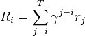
CST consists of mainly three parts;change point detection, alignment and merging. The main focus of CST is online change-point detection. The change-point detection algorithm is used to segment data into skills and uses the sum of discounted reward as the target regression variable. Each skill is assigned an appropriate abstraction. A particle filter is used to control the computational complexity of CST.

The change point detection algorithm is implemented as follows. The data for times  and models Q with prior  are given. The algorithm is assumed to be able to fit a segment from time  to  using model  with the fit probability . A linear regression model with Gaussian noise is used to compute . The Gaussian noise prior has mean zero, and variance which follows 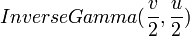. The prior for each weight follows .

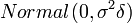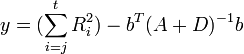
The fit probability  is computed by the following equation.

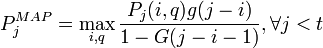
Then, CST compute the probability of the changepoint at time j with model q,  and  using an Viterbi algorithm.

The descriptions of the parameters and variables are as follows;

: a vector of m basis functions evaluated at state 

: Gamma function

: The number of basis functions q has.

: an m by m matrix with  on the diagonal and zeros else where

The skill length  is assumed to follow a Geometric distribution with parameter p

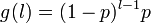
Expected skill length

Using the method above, CST can segment data into a skill chain. The time complexity of the change point detection is  and storage size is , where  is the number of particles,  is the time of computing , and there are  change points.

Next step is alignment. CST needs to align the component skills because the change-point does not occur in the exactly same places. Thus, when segmenting second trajectory after segmenting the first trajectory, it has a bias on the location of change point in the second trajectory. This bias follows a mixture of gaussians.

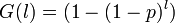
The last step is merging. CST merges skill chains into a skill tree. CST merges a pair of trajectory segments by allocating the same skill. All trajectories have the same goal and it merges two chains by starting at their final segments. If two segments are statistically similar, it merges them. This procedure is repeated until it fails to merge a pair of skill segments.  are used to determine whether a pair of trajectories are modeled better as one skill or as two different skills.

Pseudocode[edit]

The following pseudocode describes the change point detection algorithm:

  particles = [];  Process each incoming data point  for t=1:T     //Compute fit probabilities for all particles           for          p_tjq=(1-G(t-p.pos-1))*p.fit_prob*model_prior(p.model)*p.prev_MAP         p.MAP=p_tjq*g(t-p.pos)/(1-G(t-p.pos-1))     end     //Filter if necessary     if the number of particles >= N        particles=particle_filter(p.MAP, M)     end     //Determine the Viterbi path     for t==1        max_path=[]        max_MAP=1/|Q|     else        max_particle=p.MAP        max_path=max_particle.path  max_particle        max_MAP=max_particle.MAP     end     //Create new particles for a changepoint at time t     for         new_p=create_particle(model=q, pos=t, prev_MAP=max_MAP, path=max_path)        p=p  new_p     end     //Update all particles     for         particles=update_particle(current_state, current_reward,p)           end  end  //Return the most likely path to the final point  return max_path

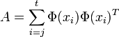
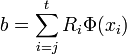
  function update_particle(current_state, current_reward, particle);  p=particle  r_t=current_reward  //Initialization  if t==0     p.A=zero matrix(p.m,p.m)     p.b=zero vector(p.m)     p.z=zero vector(p.m)     p.sum r=0     p.tr1=0     p.tr2=0  end  //Compute the basis function vector for the current state  =p.(current state)  //Update sufficient statistics  p.A=p.A+  p.z=p.z+  p.b=p.b+ p.z  p.tr1=1+  p.tr1  p.sum r=sum p.r+  p.tr1+2 p.tr2  p.tr2=p.tr2+ p.tr1  p.fit_prob=compute_fit_prob(p,v,u,delta,)

Assumptions[edit]

CTS assume that the demonstrated skills form a tree, the domain reward function is known and the best model for merging a pair of skills is the model selected for representing both individually.

Advantages[edit]

CTS is much faster learning algorithm than skill chaining. CTS can be applied to learning higher dimensional policies. Even unsuccessful episode can improve skills. Skills acquired using agent-centric features can be used for other problems.

Uses[edit]

CST has been used to acquire skills from human demonstration in the PinBall domain. It has been also used to acquire skills from human demonstration on a mobile manipulator.

References[edit]

• Konidaris, George; Scott Kuindersma; Andrew Barto ; Roderic Grupen (2010). "Constructing Skill Trees for Reinforcement Learning Agents from Demonstration Trajectories". Advances in Neural Information Processing Systems 23.

• Konidaris, George; Andrew Barto (2009). "Skill discovery in continuous reinforcement learning domains using skill chaining". Advances in Neural Information Processing Systems 22.

• Fearnhead, Paul; Zhen Liu (2007). "On-line Inference for Multiple Change Points". Journal of the Royal Statistical Society.