k-means clustering is a method of vector quantization originally from signal processing, that is popular for cluster analysis in data mining. k-means clustering aims to partition n observations into k clusters in which each observation belongs to the cluster with the nearest mean, serving as a prototype of the cluster. This results in a partitioning of the data space into Voronoi cells.
The problem is computationally difficult (NP-hard); however, there are efficient heuristic algorithms that are commonly employed and converge quickly to a local optimum. These are usually similar to theexpectation-maximization algorithm for mixtures of Gaussian distributions via an iterative refinement approach employed by both algorithms. Additionally, they both use cluster centers to model the data; however, k-means clustering tends to find clusters of comparable spatial extent, while the expectation-maximization mechanism allows clusters to have different shapes.
Contents
[hide] - 1 Description
- 2 History
- 3 Algorithms
- 3.1 Standard algorithm
- 3.1.1 Initialization methods
- 3.2 Complexity
- 3.3 Variations
- 4 Discussion
- 5 Applications
- 5.1 Vector quantization
- 5.2 Cluster analysis
- 5.3 Feature learning for (semi-)supervised classification
- 6 Relation to other statistical machine learning algorithms
- 6.1 Mean shift clustering
- 6.2 Principal component analysis (PCA)
- 6.3 Bilateral filtering
- 7 Similar problems
- 8 Software
- 8.1 Free
- 8.2 Commercial
- 8.3 Source code
- 8.4 Visualization, animation and examples
- 9 See also
- 10 References
Description[edit]
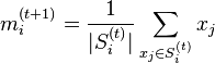
Given a set of observations (x1, x2, …, xn), where each observation is a d-dimensional real vector, k-means clustering aims to partition the n observations into k sets (k ≤ n) S = {S1, S2, …, Sk} so as to minimize the within-cluster sum of squares (WCSS):

where μi is the mean of points in Si.
History[edit]
The term "k-means" was first used by James MacQueen in 1967,[1] though the idea goes back to Hugo Steinhaus in 1957.[2] The standard algorithm was first proposed by Stuart Lloyd in 1957 as a technique for pulse-code modulation, though it wasn't published outside of Bell Labs until 1982.[3] In 1965, E.W.Forgy published essentially the same method, which is why it is sometimes referred to as Lloyd-Forgy, too.[4] A more efficient version was proposed and published in Fortran by Hartigan and Wong in 1975/1979.[5][6]
Algorithms[edit]
Standard algorithm[edit]
The most common algorithm uses an iterative refinement technique. Due to its ubiquity it is often called the k-means algorithm; it is also referred to as Lloyd's algorithm, particularly in the computer science community.
Given an initial set of k means m1(1),…,mk(1) (see below), the algorithm proceeds by alternating between two steps:[7]
- Assignment step: Assign each observation to the cluster whose mean yields the least within-cluster sum of squares (WCSS). Since the sum of squares is the squared Euclidean distance, this is intuitively the "nearest" mean.[8] (Mathematically, this means partitioning the observations according to the Voronoi diagram generated by the means).

- where each
 is assigned to exactly one
  , even if it could be is assigned to two or more of them.
- Update step: Calculate the new means to be the centroids of the observations in the new clusters.
- Since the arithmetic mean is a least-squares estimator, this also minimizes the within-cluster sum of squares (WCSS) objective.
The algorithm has converged when the assignments no longer change. Since both steps optimize the WCSS objective, and there only exists a finite number of such partitionings, the algorithm must converge to a (local) optimum. There is no guarantee that the global optimum is found using this algorithm.
The algorithm is often presented as assigning objects to the nearest cluster by distance. This is slightly inaccurate: the algorithm aims at minimizing the WCSS objective, and thus assigns by "least sum of squares". Using a different distance function other than (squared) Euclidean distance may stop the algorithm from converging. It is correct that the smallest Euclidean distance yields the smallest squared Euclidean distance and thus also yields the smallest sum of squares. Various modifications of k-means such as spherical k-means and k-medoids have been proposed to allow using other distance measures.
Initialization methods[edit]
Commonly used initialization methods are Forgy and Random Partition.[9] The Forgy method randomly chooses k observations from the data set and uses these as the initial means. The Random Partition method first randomly assigns a cluster to each observation and then proceeds to the update step, thus computing the initial mean to be the centroid of the cluster's randomly assigned points. The Forgy method tends to spread the initial means out, while Random Partition places all of them close to the center of the data set. According to Hamerly et al.,[9] the Random Partition method is generally preferable for algorithms such as the k-harmonic means and fuzzy k-means. For expectation maximization and standard k-means algorithms, the Forgy method of initialization is preferable.
- Demonstration of the standard algorithm
-
1) k initial "means" (in this casek=3) are randomly generated within the data domain (shown in color).
-
2) k clusters are created by associating every observation with the nearest mean. The partitions here represent theVoronoi diagram generated by the means.
-
3) The centroid of each of the kclusters becomes the new mean.
-
4) Steps 2 and 3 are repeated until convergence has been reached.
As it is a heuristic algorithm, there is no guarantee that it will converge to the global optimum, and the result may depend on the initial clusters. As the algorithm is usually very fast, it is common to run it multiple times with different starting conditions. However, in the worst case, k-means can be very slow to converge: in particular it has been shown that there exist certain point sets, even in 2 dimensions, on which k-means takes exponential time, that is 2Ω(n), to converge.[10] These point sets do not seem to arise in practice: this is corroborated by the fact that the smoothed running time of k-means is polynomial.[11]
The "assignment" step is also referred to as expectation step, the "update step" as maximization step, making this algorithm a variant of the generalized expectation-maximization algorithm.
Complexity[edit]
Regarding computational complexity, finding the optimal solution to the k-means clustering problem for observations in d dimensions is:
- NP-hard in general Euclidean space d even for 2 clusters [12][13]
- NP-hard for a general number of clusters k even in the plane [14]
- If k and d (the dimension) are fixed, the problem can be exactly solved in time O(ndk+1 log n), where n is the number of entities to be clustered [15]
Thus, a variety of heuristic algorithms such as Lloyds algorithm given above are generally used.
- Lloyd's
 -means algorithm has polynomial smoothed running time. It is shown that [11] for arbitrary set of
  points in
 ![[0,1]^d](http://upload.wikimedia.org/math/2/6/b/26bc47a1ae7c57f9c370dd5928d898a4.png) , if each point is independently perturbed by a normal distribution with mean
, if each point is independently perturbed by a normal distribution with mean  and variance
  , then the expected running time of-means algorithm is bounded by
 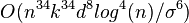 , which is a polynomial in , ,
  and
and  .
.
- Better bounds are proved for simple cases. For example,[16] showed that the running time of -means algorithm is bounded by
 for points in an integer lattice
 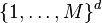 .
.
Variations[edit]
- k-medians clustering uses the median in each dimension instead of the mean, and this way minimizes
 norm (Taxicab geometry).
 - k-medoids (also: Partitioning Around Medoids, PAM) uses the medoid instead of the mean, and this way minimizes the sum of distances for arbitrary distance functions.
- Fuzzy C-Means Clustering is a soft version of K-means, where each data point has a fuzzy degree of belonging to each cluster.
- Gaussian mixture models trained with expectation-maximization algorithm (EM algorithm) maintains probabilistic assignments to clusters, instead of deterministic assignments, and multivariate Gaussian distributions instead of means.
- Several methods have been proposed to choose better starting clusters. One recent proposal is k-means++.
- The filtering algorithm uses kd-trees to speed up each k-means step.[17]
- Some methods attempt to speed up each k-means step using coresets[18] or the triangle inequality.[19]
- Escape local optima by swapping points between clusters.[6]
Discussion[edit]

A typical example of the k-means convergence to a local minimum. In this example, the result of k-means clustering (the right figure) contradicts the obvious cluster structure of the data set. The small circles are the data points, the four ray stars are the centroids (means). The initial configuration is on the left figure. The algorithm converges after five iterations presented on the figures, from the left to the right. The illustration was prepared with the Mirkes Java applet.
[22]
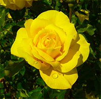
k-means clustering result for the
Iris flower data set and actual species visualized using
ELKI. Cluster means are marked using larger, semi-transparent symbols.

k-means clustering and EM clustering on an artificial dataset ("mouse"). The tendency of
k-means to produce equi-sized clusters leads to bad results, while EM benefits from the Gaussian distribution present in the data set
The two key features of k-means which make it efficient are often regarded as its biggest drawbacks:
- Euclidean distance is used as a metric and variance is used as a measure of cluster scatter.
- The number of clusters k is an input parameter: an inappropriate choice of k may yield poor results. That is why, when performing k-means, it is important to run diagnostic checks for determining the number of clusters in the data set.
- Convergence to a local minimum may produce counterintuitive ("wrong") results (see example in Fig.).
A key limitation of k-means is its cluster model. The concept is based on spherical clusters that are separable in a way so that the mean value converges towards the cluster center. The clusters are expected to be of similar size, so that the assignment to the nearest cluster center is the correct assignment. When for example applying k-means with a value of  onto the well-known Iris flower data set, the result often fails to separate the three Iris species contained in the data set. With
  , the two visible clusters (one containing two species) will be discovered, whereas with one of the two clusters will be split into two even parts. In fact, is more appropriate for this data set, despite the data set containing 3 classes. As with any other clustering algorithm, the k-means result relies on the data set to satisfy the assumptions made by the clustering algorithms. It works well on some data sets, while failing on others.
The result of k-means can also be seen as the Voronoi cells of the cluster means. Since data is split halfway between cluster means, this can lead to suboptimal splits as can be seen in the "mouse" example. The Gaussian models used by the Expectation-maximization algorithm (which can be seen as a generalization of k-means) are more flexible here by having both variances and covariances. The EM result is thus able to accommodate clusters of variable size much better than k-means as well as correlated clusters (not in this example).
Applications[edit]
k-means clustering in particular when using heuristics such as Lloyd's algorithm is rather easy to implement and apply even on large data sets. As such, it has been successfully used in various topics, ranging from market segmentation, computer vision, geostatistics,[23] and astronomy to agriculture. It often is used as a preprocessing step for other algorithms, for example to find a starting configuration.
Vector quantization[edit]
Two-channel (for illustration purposes -- red and green only) color image.

Vector quantization of colors present in the image above into Voronoi cells using
k-means.
k-means originates from signal processing, and still finds use in this domain. For example in computer graphics, color quantization is the task of reducing the color palette of an image to a fixed number of colors k. The k-means algorithm can easily be used for this task and produces competitive results. Other uses of vector quantization includenon-random sampling, as k-means can easily be used to choose k different but prototypical objects from a large data set for further analysis.
Cluster analysis[edit]
In cluster analysis, the k-means algorithm can be used to partition the input data set into k partitions (clusters).
However, the pure k-means algorithm is not very flexible, and as such of limited use (except for when vector quantization as above is actually the desired use case!). In particular, the parameter k is known to be hard to choose (as discussed below) when not given by external constraints. In contrast to other algorithms, k-means can also not be used with arbitrary distance functions or be use on non-numerical data. For these use cases, many other algorithms have been developed since.
Feature learning for (semi-)supervised classification[edit]
k-means clustering has been used as a feature learning (or dictionary learning) step for (semi-)supervised learning.[24] In this usage, clustering is performed on a large dataset, which need to be labeled. Then supervised learning is performed, and for each labeled sample, the distance to each of the k learned cluster centroids is computed to induce k extra features for the sample. The feature can be a boolean with value 1 for the closest centroid,[25] or some smooth transformation of the distance.[26] By transforming the sample-cluster distance through a Gaussian RBF, one effectively obtains the hidden layer of a radial basis function network.[27]
This use of k-means has been successfully combined with simple, linear classifiers for semi-supervised learning in NLP (specifically for named entity recognition)[28] and in computer vision. On an object recognition task, it was found to exhibit comparable performance with more sophisticated feature learning approaches such as autoencoders and restricted Boltzmann machines.[26]
Relation to other statistical machine learning algorithms[edit]
k-means clustering, and its associated expectation-maximization algorithm, is a special case of a Gaussian mixture model, specifically, the limit of taking all covariances as diagonal, equal, and small. It is often easy to generalize a k-means problem into a Gaussian mixture model.[29]
Mean shift clustering[edit]
Basic mean shift clustering algorithms maintain a set of data points the same size as the input data set. Initially, this set is copied from the input set. Then this set is iteratively replaced by the mean of those points in the set that are within a given distance of that point. By contrast, k-means restricts this updated set to k points usually much less than the number of points in the input data set, and replaces each point in this set by the mean of all points in the input set that are closer to that point than any other (e.g. within the Voronoi partition of each updating point). A mean shift algorithm that is similar then to k-means, called likelihood mean shift, replaces the set of points undergoing replacement by the mean of all points in the input set that are within a given distance of the changing set.[30] One of the advantages of mean shift over k-means is that there is no need to choose the number of clusters, because mean shift is likely to find only a few clusters if indeed only a small number exist. However, mean shift can be much slower than k-means, and still requires selection of a bandwidth parameter. Mean shift has soft variants much as k-means does.
Principal component analysis (PCA)[edit]
It was asserted in [31][32] that the relaxed solution of k-means clustering, specified by the cluster indicators, is given by the PCA (principal component analysis) principal components, and the PCA subspace spanned by the principal directions is identical to the cluster centroid subspace. However, that PCA is a useful relaxation of k-means clustering was not a new result (see, for example,[33]), and it is straightforward to uncover counterexamples to the statement that the cluster centroid subspace is spanned by the principal directions.
Bilateral filtering[edit]
k-means implicitly assumes that the ordering of the input data set does not matter. The bilateral filter is similar to K-means and mean shift in that it maintains a set of data points that are iteratively replaced by means. However, the bilateral filter restricts the calculation of the (kernel weighted) mean to include only points that are close in the ordering of the input data.[30] This makes it applicable to problems such as image denoising, where the spatial arrangement of pixels in an image is of critical importance.
Similar problems[edit]
The set of squared error minimizing cluster functions also includes the k-medoids algorithm, an approach which forces the center point of each cluster to be one of the actual points, i.e., it uses medoids in place of centroids.
Software[edit]
Commercial[edit]
Source code[edit]
- ELKI and Weka are written in Java and include k-means and variations
- K-means application in PHP,[34] using VB,[35] using Perl,[36] using C++,[37] using Matlab,[38] using Ruby,[39][40] using Python with scipy,[41] using X10[42]
- A parallel out-of-core implementation in C[43]
- An open-source collection of clustering algorithms, including k-means, implemented in Javascript.[44] Online demo.[45]
Visualization, animation and examples[edit]
See also[edit]
References[edit]
- ^ Jump up to:a b MacQueen, J. B. (1967). "Some Methods for classification and Analysis of Multivariate Observations". Proceedings of 5th Berkeley Symposium on Mathematical Statistics and Probability 1. University of California Press. pp. 281–297. MR 0214227.Zbl 0214.46201. Retrieved 2009-04-07.
- Jump up^ Steinhaus, H. (1957). "Sur la division des corps matériels en parties". Bull. Acad. Polon. Sci. (in French) 4 (12): 801–804.MR 0090073. Zbl 0079.16403.
- ^ Jump up to:a b Lloyd, S. P. (1957). "Least square quantization in PCM". Bell Telephone Laboratories Paper. Published in journal much later:Lloyd., S. P. (1982). "Least squares quantization in PCM". IEEE Transactions on Information Theory 28 (2): 129–137.doi:10.1109/TIT.1982.1056489. Retrieved 2009-04-15.
- Jump up^ E.W. Forgy (1965). "Cluster analysis of multivariate data: efficiency versus interpretability of classifications". Biometrics 21: 768–769.
- Jump up^ J.A. Hartigan (1975). Clustering algorithms. John Wiley & Sons, Inc.
- ^ Jump up to:a b c Hartigan, J. A.; Wong, M. A. (1979). "Algorithm AS 136: A K-Means Clustering Algorithm". Journal of the Royal Statistical Society, Series C 28 (1): 100–108. JSTOR 2346830.
- Jump up^ MacKay, David (2003). "Chapter 20. An Example Inference Task: Clustering". Information Theory, Inference and Learning Algorithms. Cambridge University Press. pp. 284–292. ISBN 0-521-64298-1. MR 2012999.
- Jump up^ Since the square root is a monotone function, this also is the minimum Euclidean distance assignment.
- ^ Jump up to:a b Hamerly, G. and Elkan, C. (2002). "Alternatives to the k-means algorithm that find better clusterings". Proceedings of the eleventh international conference on Information and knowledge management (CIKM).
- Jump up^ Vattani., A. (2011). "k-means requires exponentially many iterations even in the plane". Discrete and Computational Geometry 45 (4): 596–616. doi:10.1007/s00454-011-9340-1.
- ^ Jump up to:a b Arthur, D.; Manthey, B.; Roeglin, H. (2009). "k-means has polynomial smoothed complexity". Proceedings of the 50th Symposium on Foundations of Computer Science (FOCS).
- Jump up^ Aloise, D.; Deshpande, A.; Hansen, P.; Popat, P. (2009). "NP-hardness of Euclidean sum-of-squares clustering". Machine Learning 75: 245–249. doi:10.1007/s10994-009-5103-0.
- Jump up^ Dasgupta, S. and Freund, Y. (July 2009). "Random Projection Trees for Vector Quantization". Information Theory, IEEE Transactions on 55: 3229–3242. arXiv:0805.1390. doi:10.1109/TIT.2009.2021326.
- Jump up^ Mahajan, M.; Nimbhorkar, P.; Varadarajan, K. (2009). "The Planar k-Means Problem is NP-Hard". Lecture Notes in Computer Science 5431: 274–285. doi:10.1007/978-3-642-00202-1_24.
- Jump up^ Inaba, M.; Katoh, N.; Imai, H. (1994). "Applications of weighted Voronoi diagrams and randomization to variance-based k-clustering". Proceedings of 10th ACM Symposium on Computational Geometry. pp. 332–339. doi:10.1145/177424.178042.
- Jump up^ Arthur; Abhishek Bhowmick (2009). A theoretical analysis of Lloyd's algorithm for k-means clustering (Thesis).[1][dead link]
- Jump up^ Kanungo, T.; Mount, D. M.; Netanyahu, N. S.; Piatko, C. D.; Silverman, R.; Wu, A. Y. (2002). "An efficient k-means clustering algorithm: Analysis and implementation". IEEE Trans. Pattern Analysis and Machine Intelligence 24: 881–892.doi:10.1109/TPAMI.2002.1017616. Retrieved 2009-04-24.
- Jump up^ Frahling, G.; Sohler, C. (2006). "A fast k-means implementation using coresets". Proceedings of the twenty-second annual symposium on Computational geometry (SoCG).
- Jump up^ Elkan, C. (2003). "Using the triangle inequality to accelerate k-means". Proceedings of the Twentieth International Conference on Machine Learning (ICML).
- Jump up^ Dhillon, I. S.; Modha, D. M. (2001). "Concept decompositions for large sparse text data using clustering". Machine Learning 42(1): 143–175.
- Jump up^ Amorim, R. C.; Mirkin, B (2012). "Minkowski metric, feature weighting and anomalous cluster initializing in K-Means clustering".Pattern Recognition 45 (3): 1061–1075. doi:10.1016/j.patcog.2011.08.012.
- ^ Jump up to:a b E.M. Mirkes, K-means and K-medoids applet. University of Leicester, 2011.
- Jump up^ Honarkhah, M and Caers, J, 2010, Stochastic Simulation of Patterns Using Distance-Based Pattern Modeling, Mathematical Geosciences, 42: 487 - 517
- Jump up^ Coates, Adam; Ng, Andrew Y. (2012). "Learning feature representations with k-means". In G. Montavon, G. B. Orr, K.-R. Müller. Neural Networks: Tricks of the Trade. Springer.
- Jump up^ Csurka, Gabriella; Dance, Christopher C.; Fan, Lixin; Willamowski, Jutta; Bray, Cédric (2004). "Visual categorization with bags of keypoints". ECCV Workshop on Statistical Learning in Computer Vision.
- ^ Jump up to:a b Coates, Adam; Lee, Honglak; Ng, Andrew Y. (2011). "An analysis of single-layer networks in unsupervised feature learning". International Conference on Artificial Intelligence and Statistics (AISTATS).
- Jump up^ Schwenker, Friedhelm; Kestler, Hans A.; Palm, Günther (2001). "Three learning phases for radial-basis-function networks".Neural Networks 14: 439–458.
- Jump up^ Lin, Dekang; Wu, Xiaoyun (2009). "Phrase clustering for discriminative learning". Annual Meeting of the ACL and IJCNLP. pp. 1030–1038.
- Jump up^ Press, WH; Teukolsky, SA; Vetterling, WT; Flannery, BP (2007). "Section 16.1. Gaussian Mixture Models and k-Means Clustering". Numerical Recipes: The Art of Scientific Computing (3rd ed.). New York: Cambridge University Press. ISBN 978-0-521-88068-8.
- ^ Jump up to:a b Little, M.A.; Jones, N.S. (2011). "Generalized Methods and Solvers for Piecewise Constant Signals: Part I". Proceedings of the Royal Society A.
- Jump up^ H. Zha, C. Ding, M. Gu, X. He and H.D. Simon (Dec. 2001). "Spectral Relaxation for K-means Clustering". Neural Information Processing Systems vol.14 (NIPS 2001) (Vancouver, Canada): 1057–1064.
- Jump up^ Chris Ding and Xiaofeng He (July 2004). "K-means Clustering via Principal Component Analysis". Proc. of Int'l Conf. Machine Learning (ICML 2004): 225–232.
- Jump up^ Drineas, P.; A. Frieze, R. Kannan, S. Vempala, V. Vinay (2004). "Clustering large graphs via the singular value decomposition". Machine learning 56: 9–33. Retrieved 2012-08-02.
- Jump up^ http://www25.brinkster.com/denshade/kmeans.php.htm
- Jump up^ K-Means Clustering Tutorial: Download
- Jump up^ Perl script for Kmeans clustering
- Jump up^ Antonio Gulli's coding playground: K-means in C
- Jump up^ K-Means Clustering Tutorial: Matlab Code
- Jump up^ AI4R :: Artificial Intelligence for Ruby
- Jump up^ reddavis/K-Means · GitHub
- Jump up^ K-means clustering and vector quantization (scipy.cluster.vq) — SciPy v0.11 Reference Guide (DRAFT)
- Jump up^ http://dist.codehaus.org/x10/applications/samples/KMeansDist.x10
- Jump up^ http://www.cs.princeton.edu/~wdong/kmeans/
- Jump up^ http://code.google.com/p/figue/ FIGUE
- Jump up^ http://web.science.mq.edu.au/~jydelort/figue/demo.html
- Jump up^ Clustering - K-means demo
- Jump up^ siebn.de - YAK-Means
- Jump up^ k-Means and Voronoi Tesselation: Built with Processing | Information & Visualization
- Jump up^ Hyper-threaded Java - JavaWorld
- Jump up^ Color clustering
- Jump up^ Interactive step-by-step examples in Javascript of good and bad k-means clustering
- Jump up^ Clustergram: visualization and diagnostics for cluster analysis (R code) | R-statistics blog