In machine learning, the perceptron is an algorithm for supervisedclassification of an input into one of several possible non-binary outputs. It is a type of linear classifier, i.e. a classification algorithm that makes its predictions based on a linear predictor function combining a set of weights with the feature vector describing a given input using the delta rule. The learning algorithm for perceptrons is an online algorithm, in that it processes elements in the training set one at a time.
The perceptron algorithm was invented in 1957 at the Cornell Aeronautical Laboratory by Frank Rosenblatt.[1]
Definition[edit]
The perceptron is a binary classifier which maps its input  (a real-valuedvector) to an output value
  (a single binary value):
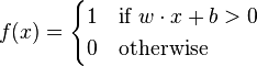
where  is a vector of real-valued weights,
  is the dot product (which here computes a weighted sum), and
  is the 'bias', a constant term that does not depend on any input value.
The value of (0 or 1) is used to classify as either a positive or a negative instance, in the case of a binary classification problem. If is negative, then the weighted combination of inputs must produce a positive value greater than  in order to push the classifier neuron over the 0 threshold. Spatially, the bias alters the position (though not the orientation) of the decision boundary. The perceptron learning algorithm does not terminate if the learning set is not linearly separable. If the vectors are not linearly separable learning will never reach a point where all vectors are classified properly. The most famous example of the perceptron's inability to solve problems with linearly nonseparable vectors is the Boolean exclusive-or problem. The solution spaces of decision boundaries for all binary functions and learning behaviors are studied in the reference.[2]
In the context of artificial neural networks, a perceptron is an artificial neuron using the Heaviside step function as the activation function. The perceptron algorithm is also termed the single-layer perceptron, to distinguish it from amultilayer perceptron, which is a misnomer for a more complicated neural network. As a linear classifier, the single-layer perceptron is the simplest feedforward neural network.
Learning algorithm[edit]
Below is an example of a learning algorithm for a (single-layer) perceptron. For multilayer perceptrons, where a hidden layer exists, more sophisticated algorithms such as backpropagation must be used. Alternatively, methods such as thedelta rule can be used if the function is non-linear and differentiable, although the one below will work as well.
When multiple perceptrons are combined in an artificial neural network, each output neuron operates independently of all the others; thus, learning each output can be considered in isolation.
Definitions[edit]
We first define some variables:
 denotes the output from the perceptron for an input vector
  .
. is the bias term, which in the example below we take to be 0.
 is the training set of
  samples, where:
  is the
  -dimensional input vector.
 is the desired output value of the perceptron for that input.
We show the values of the nodes as follows:
 is the value of the
  th node of the
  th training input vector.
 .
.
To represent the weights:
 is the th value in the weight vector, to be multiplied by the value of the th input node.
An extra dimension, with index  , can be added to all input vectors, with
  , in which case
  replaces the bias term. To show the time-dependence of
  , we use:
 is the weight at time
  .
. is the learning rate, where
  .
.
Too high a learning rate makes the perceptron periodically oscillate around the solution unless additional steps are taken.

The appropriate weights are applied to the inputs, and the resulting weighted sum passed to a function that produces the output y.
1. Initialise the weights and the threshold. Weights may be initialised to 0 or to a small random value. In the example below, we use 0.
2. For each example  in our training set
  , perform the following steps over the input
  and desired output :
- 2a. Calculate the actual output:
![y_j(t) = f[\mathbf{w}(t)\cdot\mathbf{x}_j] = f[w_0(t) + w_1(t)x_{j,1} + w_2(t)x_{j,2} + \dotsb + w_n(t)x_{j,n}]](http://upload.wikimedia.org/math/8/d/6/8d668363ae3e091a1df521b8e86b6577.png)
- 2b. Update the weights:
 , for all nodes
  .
.
3. Repeat Step 2 until the iteration error ![\frac{1}{s} \sum_j^s [d_j - y_j(t)] \,](http://upload.wikimedia.org/math/5/e/f/5efa38a3f4a0ca2de5d91799e5e5ba25.png) is less than a user-specified error threshold
is less than a user-specified error threshold  , or a predetermined number of iterations have been completed.
The algorithm updates the weights immediately after steps 2a and 2b are applied to a pair in the training set rather than waiting until all pairs in the training set have undergone these steps.
Convergence[edit]
The training set  is said to be linearly separable if the positive examples can be separated from the negative examples by a hyperplane; that is, if there exists a positive constant
  and a weight vector such that
 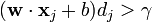 for all
  . That is, if we say that is the weight vector to the perceptron, then the output of the perceptron,
  , multiplied by the desired output of the perceptron,
  , must be greater than the positive constant, , for all input-vector/output-value pairs
  in
in  .
.
Novikoff (1962) proved that the perceptron algorithm converges after a finite number of iterations if the data set is linearly separable. The idea of the proof is that the weight vector is always adjusted by a bounded amount in a direction that it has a negative dot product with, and thus can be bounded above by  where t is the number of changes to the weight vector. But it can also be bounded below by
  because if there exists an (unknown) satisfactory weight vector, then every change makes progress in this (unknown) direction by a positive amount that depends only on the input vector. This can be used to show that the number t of updates to the weight vector is bounded by
  , where R is the maximum norm of an input vector.
However, if the training set is not linearly separable, the above online algorithm will not converge.
The decision boundary of a perceptron is invariant with respect to scaling of the weight vector; that is, a perceptron trained with initial weight vector and learning rate behaves identically to a perceptron trained with initial weight vector  and learning rate 1. Thus, since the initial weights become irrelevant with increasing number of iterations, the learning rate does not matter in the case of the perceptron and is usually just set to 1.
Variants[edit]
The pocket algorithm with ratchet (Gallant, 1990) solves the stability problem of perceptron learning by keeping the best solution seen so far "in its pocket". The pocket algorithm then returns the solution in the pocket, rather than the last solution. It can be used also for non-separable data sets, where the aim is to find a perceptron with a small number of misclassifications.
In separable problems, perceptron training can also aim at finding the largest separating margin between the classes. The so-called perceptron of optimal stability can be determined by means of iterative training and optimization schemes, such as the Min-Over algorithm (Krauth and Mezard, 1987)[3] or the AdaTron (Anlauf and Biehl, 1989)) .[4] AdaTron uses the fact that the corresponding quadratic optimization problem is convex. The perceptron of optimal stability, together with thekernel trick, are the conceptual foundations of the support vector machine.
The  -perceptron further used a pre-processing layer of fixed random weights, with thresholded output units. This enabled the perceptron to classify analogue patterns, by projecting them into a binary space. In fact, for a projection space of sufficiently high dimension, patterns can become linearly separable.
For example, consider the case of having to classify data into two classes. Here is a small such data set, consisting of two points coming from two Gaussian distributions.
-
-
A linear classifier operating on the original space
-
A linear classifier operating on a high-dimensional projection
A linear classifier can only separate points with a hyperplane, so no linear classifier can classify all the points here perfectly. On the other hand, the data can be projected into a large number of dimensions. In our example, a random matrix was used to project the data linearly to a 1000-dimensional space; then each resulting data point was transformed through the hyperbolic tangent function. A linear classifier can then separate the data, as shown in the third figure. However the data may still not be completely separable in this space, in which the perceptron algorithm would not converge. In the example shown, stochastic steepest gradient descent was used to adapt the parameters.
Furthermore, by adding nonlinear layers between the input and output, one can separate all data, and can model any well-defined function to arbitrary precision given enough training data. This model is a generalization known as a multilayer perceptron.
Another way to solve nonlinear problems without using multiple layers is to use higher order networks (sigma-pi unit). In this type of network, each element in the input vector is extended with each pairwise combination of multiplied inputs (second order). This can be extended to an n-order network.
It should be kept in mind, however, that the best classifier is not necessarily that which classifies all the training data perfectly. Indeed, if we had the prior constraint that the data come from equi-variant Gaussian distributions, the linear separation in the input space is optimal.
Other linear classification algorithms include Winnow, support vector machine and logistic regression.
Example[edit]
A perceptron learns to perform a binary NAND function on inputs  and
and  .
.
Inputs:  , , , with input held constant at 1.
Threshold (): 0.5
Bias (): 0
Learning rate ( ): 0.1
Training set, consisting of four samples: 
In the following, the final weights of one iteration become the initial weights of the next. Each cycle over all the samples in the training set is demarcated with heavy lines.
| Input | Initial weights | Output | Error | Correction | Final weights |
| Sensor values | Desired output | Per sensor | Sum | Network |
 |  |  |  |  |  |  |  |  |  | | |  |  | | | |
 | | |  |  |  |  | if  then 1, else 0 then 1, else 0 |  |  |  |  |  |
| 1 | 0 | 0 | 1 | 0 | 0 | 0 | 0 | 0 | 0 | 0 | 0 | 1 | +0.1 | 0.1 | 0 | 0 |
| 1 | 0 | 1 | 1 | 0.1 | 0 | 0 | 0.1 | 0 | 0 | 0.1 | 0 | 1 | +0.1 | 0.2 | 0 | 0.1 |
| 1 | 1 | 0 | 1 | 0.2 | 0 | 0.1 | 0.2 | 0 | 0 | 0.2 | 0 | 1 | +0.1 | 0.3 | 0.1 | 0.1 |
| 1 | 1 | 1 | 0 | 0.3 | 0.1 | 0.1 | 0.3 | 0.1 | 0.1 | 0.5 | 0 | 0 | 0 | 0.3 | 0.1 | 0.1 |
| 1 | 0 | 0 | 1 | 0.3 | 0.1 | 0.1 | 0.3 | 0 | 0 | 0.3 | 0 | 1 | +0.1 | 0.4 | 0.1 | 0.1 |
| 1 | 0 | 1 | 1 | 0.4 | 0.1 | 0.1 | 0.4 | 0 | 0.1 | 0.5 | 0 | 1 | +0.1 | 0.5 | 0.1 | 0.2 |
| 1 | 1 | 0 | 1 | 0.5 | 0.1 | 0.2 | 0.5 | 0.1 | 0 | 0.6 | 1 | 0 | 0 | 0.5 | 0.1 | 0.2 |
| 1 | 1 | 1 | 0 | 0.5 | 0.1 | 0.2 | 0.5 | 0.1 | 0.2 | 0.8 | 1 | -1 | -0.1 | 0.4 | 0 | 0.1 |
| 1 | 0 | 0 | 1 | 0.4 | 0 | 0.1 | 0.4 | 0 | 0 | 0.4 | 0 | 1 | +0.1 | 0.5 | 0 | 0.1 |
| 1 | 0 | 1 | 1 | 0.5 | 0 | 0.1 | 0.5 | 0 | 0.1 | 0.6 | 1 | 0 | 0 | 0.5 | 0 | 0.1 |
| 1 | 1 | 0 | 1 | 0.5 | 0 | 0.1 | 0.5 | 0 | 0 | 0.5 | 0 | 1 | +0.1 | 0.6 | 0.1 | 0.1 |
| 1 | 1 | 1 | 0 | 0.6 | 0.1 | 0.1 | 0.6 | 0.1 | 0.1 | 0.8 | 1 | -1 | -0.1 | 0.5 | 0 | 0 |
| 1 | 0 | 0 | 1 | 0.5 | 0 | 0 | 0.5 | 0 | 0 | 0.5 | 0 | 1 | +0.1 | 0.6 | 0 | 0 |
| 1 | 0 | 1 | 1 | 0.6 | 0 | 0 | 0.6 | 0 | 0 | 0.6 | 1 | 0 | 0 | 0.6 | 0 | 0 |
| 1 | 1 | 0 | 1 | 0.6 | 0 | 0 | 0.6 | 0 | 0 | 0.6 | 1 | 0 | 0 | 0.6 | 0 | 0 |
| 1 | 1 | 1 | 0 | 0.6 | 0 | 0 | 0.6 | 0 | 0 | 0.6 | 1 | -1 | -0.1 | 0.5 | -0.1 | -0.1 |
| 1 | 0 | 0 | 1 | 0.5 | -0.1 | -0.1 | 0.5 | 0 | 0 | 0.5 | 0 | 1 | +0.1 | 0.6 | -0.1 | -0.1 |
| 1 | 0 | 1 | 1 | 0.6 | -0.1 | -0.1 | 0.6 | 0 | -0.1 | 0.5 | 0 | 1 | +0.1 | 0.7 | -0.1 | 0 |
| 1 | 1 | 0 | 1 | 0.7 | -0.1 | 0 | 0.7 | -0.1 | 0 | 0.6 | 1 | 0 | 0 | 0.7 | -0.1 | 0 |
| 1 | 1 | 1 | 0 | 0.7 | -0.1 | 0 | 0.7 | -0.1 | 0 | 0.6 | 1 | -1 | -0.1 | 0.6 | -0.2 | -0.1 |
| 1 | 0 | 0 | 1 | 0.6 | -0.2 | -0.1 | 0.6 | 0 | 0 | 0.6 | 1 | 0 | 0 | 0.6 | -0.2 | -0.1 |
| 1 | 0 | 1 | 1 | 0.6 | -0.2 | -0.1 | 0.6 | 0 | -0.1 | 0.5 | 0 | 1 | +0.1 | 0.7 | -0.2 | 0 |
| 1 | 1 | 0 | 1 | 0.7 | -0.2 | 0 | 0.7 | -0.2 | 0 | 0.5 | 0 | 1 | +0.1 | 0.8 | -0.1 | 0 |
| 1 | 1 | 1 | 0 | 0.8 | -0.1 | 0 | 0.8 | -0.1 | 0 | 0.7 | 1 | -1 | -0.1 | 0.7 | -0.2 | -0.1 |
| 1 | 0 | 0 | 1 | 0.7 | -0.2 | -0.1 | 0.7 | 0 | 0 | 0.7 | 1 | 0 | 0 | 0.7 | -0.2 | -0.1 |
| 1 | 0 | 1 | 1 | 0.7 | -0.2 | -0.1 | 0.7 | 0 | -0.1 | 0.6 | 1 | 0 | 0 | 0.7 | -0.2 | -0.1 |
| 1 | 1 | 0 | 1 | 0.7 | -0.2 | -0.1 | 0.7 | -0.2 | 0 | 0.5 | 0 | 1 | +0.1 | 0.8 | -0.1 | -0.1 |
| 1 | 1 | 1 | 0 | 0.8 | -0.1 | -0.1 | 0.8 | -0.1 | -0.1 | 0.6 | 1 | -1 | -0.1 | 0.7 | -0.2 | -0.2 |
| 1 | 0 | 0 | 1 | 0.7 | -0.2 | -0.2 | 0.7 | 0 | 0 | 0.7 | 1 | 0 | 0 | 0.7 | -0.2 | -0.2 |
| 1 | 0 | 1 | 1 | 0.7 | -0.2 | -0.2 | 0.7 | 0 | -0.2 | 0.5 | 0 | 1 | +0.1 | 0.8 | -0.2 | -0.1 |
| 1 | 1 | 0 | 1 | 0.8 | -0.2 | -0.1 | 0.8 | -0.2 | 0 | 0.6 | 1 | 0 | 0 | 0.8 | -0.2 | -0.1 |
| 1 | 1 | 1 | 0 | 0.8 | -0.2 | -0.1 | 0.8 | -0.2 | -0.1 | 0.5 | 0 | 0 | 0 | 0.8 | -0.2 | -0.1 |
| 1 | 0 | 0 | 1 | 0.8 | -0.2 | -0.1 | 0.8 | 0 | 0 | 0.8 | 1 | 0 | 0 | 0.8 | -0.2 | -0.1 |
| 1 | 0 | 1 | 1 | 0.8 | -0.2 | -0.1 | 0.8 | 0 | -0.1 | 0.7 | 1 | 0 | 0 | 0.8 | -0.2 | -0.1 |
This example can be implemented in the following Python code.
threshold = 0.5learning_rate = 0.1weights = [0, 0, 0]training_set = [((1, 0, 0), 1), ((1, 0, 1), 1), ((1, 1, 0), 1), ((1, 1, 1), 0)] def dot_product(values, weights): return sum(value * weight for value, weight in zip(values, weights)) while True: print('-' * 60) error_count = 0 for input_vector, desired_output in training_set: print(weights) result = dot_product(input_vector, weights) > threshold error = desired_output - result if error != 0: error_count += 1 for index, value in enumerate(input_vector): weights[index] += learning_rate * error * value if error_count == 0: breakMulticlass perceptron[edit]
Like most other techniques for training linear classifiers, the perceptron generalizes naturally to multiclass classification. Here, the input and the output  are drawn from arbitrary sets. A feature representation function
  maps each possible input/output pair to a finite-dimensional real-valued feature vector. As before, the feature vector is multiplied by a weight vector , but now the resulting score is used to choose among many possible outputs:

Learning again iterates over the examples, predicting an output for each, leaving the weights unchanged when the predicted output matches the target, and changing them when it does not. The update becomes:

This multiclass formulation reduces to the original perceptron when is a real-valued vector, is chosen from  , and
, and  .
.
For certain problems, input/output representations and features can be chosen so that  can be found efficiently even though is chosen from a very large or even infinite set.
In recent years, perceptron training has become popular in the field of natural language processing for such tasks as part-of-speech tagging and syntactic parsing (Collins, 2002).
History[edit]
- See also: History of artificial intelligence, AI winter and Frank Rosenblatt
Although the perceptron initially seemed promising, it was eventually proved that perceptrons could not be trained to recognise many classes of patterns. This led to the field of neural network research stagnating for many years, before it was recognised that a feedforward neural network with two or more layers (also called a multilayer perceptron) had far greater processing power than perceptrons with one layer (also called a single layer perceptron). Single layer perceptrons are only capable of learning linearly separable patterns; in 1969 a famous book entitled Perceptrons by Marvin Minsky andSeymour Papert showed that it was impossible for these classes of network to learn an XOR function. It is often believed that they also conjectured (incorrectly) that a similar result would hold for a multi-layer perceptron network. However, this is not true, as both Minsky and Papert already knew that multi-layer perceptrons were capable of producing an XOR Function. (See the page on Perceptrons for more information.) Three years later Stephen Grossberg published a series of papers introducing networks capable of modelling differential, contrast-enhancing and XOR functions. (The papers were published in 1972 and 1973, see e.g.: Grossberg, Contour enhancement, short-term memory, and constancies in reverberating neural networks. Studies in Applied Mathematics, 52 (1973), 213-257, online [1]). Nevertheless the often-miscited Minsky/Papert text caused a significant decline in interest and funding of neural network research. It took ten more years until neural network research experienced a resurgence in the 1980s. This text was reprinted in 1987 as "Perceptrons - Expanded Edition" where some errors in the original text are shown and corrected.
The kernel Perceptron algorithm was already introduced in 1964 by Aizerman et al.[5] Margin bounds guarantees were given for the Perceptron algorithm in the general non-separable case first by Freund and Schapire (1998),[6] and more recently by Mohri and Rostamizadeh (2013) who extend previous results and give new L1 bounds.[7] The kernel Perceptron algorithm is commonly used in natural language processing applications[8] and to large-scale machine learning problems in a distributed computing setting.[9]
References[edit]
- ^ Rosenblatt, Frank (1957), The Perceptron--a perceiving and recognizing automaton. Report 85-460-1, Cornell Aeronautical Laboratory.
- ^ Liou, D.-R.; Liou, J.-W.; Liou, C.-Y. (2013). "Learning Behaviors of Perceptron". ISBN 978-1-477554-73-9. iConcept Press.
- ^ W. Krauth and M. Mezard. Learning algorithms with optimal stabilty in neural networks. J. of Physics A: Math. Gen. 20: L745-L752 (1987)
- ^ J.K. Anlauf and M. Biehl. The AdaTron: an Adaptive Perceptron algorithm. Europhysics Letters 10: 687-692 (1989)
- ^ M. A. Aizerman, E. M. Braverman, and L. I. Rozonoer. Theoretical foundations of the potential function method in pattern recognition learning. Automation and Remote Control, 25:821–837, 1964
- ^ Freund, Y. and Schapire, R. E. 1998. Large margin classification using the perceptron algorithm. In Proceedings of the 11th Annual Conference on Computational Learning Theory (COLT' 98). ACM Press.
- ^ Mohri, Mehryar and Rostamizadeh, Afshin (2013). Perceptron Mistake Bounds arXiv:1305.0208, 2013.
- ^ Collins, M. 2002. Discriminative training methods for hidden Markov models: Theory and experiments with the perceptron algorithm in Proceedings of the Conference on Empirical Methods in Natural Language Processing (EMNLP '02)
- ^ McDonald, R., Hall, K., & Mann, G. (2010). Distributed Training Strategies for the Structured Perceptron. pp. 456-464. Association for Computational Linguistics.
- Aizerman, M. A. and Braverman, E. M. and Lev I. Rozonoer. Theoretical foundations of the potential function method in pattern recognition learning. Automation and Remote Control, 25:821–837, 1964.
- Rosenblatt, Frank (1958), The Perceptron: A Probabilistic Model for Information Storage and Organization in the Brain, Cornell Aeronautical Laboratory, Psychological Review, v65, No. 6, pp. 386–408. doi:10.1037/h0042519.
- Rosenblatt, Frank (1962), Principles of Neurodynamics. Washington, DC:Spartan Books.
- Minsky M. L. and Papert S. A. 1969. Perceptrons. Cambridge, MA: MIT Press.
- Freund, Y. and Schapire, R. E. 1998. Large margin classification using the perceptron algorithm. In Proceedings of the 11th Annual Conference on Computational Learning Theory (COLT' 98). ACM Press.
- Freund, Y. and Schapire, R. E. 1999. Large margin classification using the perceptron algorithm. In Machine Learning 37(3):277-296, 1999.
- Gallant, S. I. (1990). Perceptron-based learning algorithms. IEEE Transactions on Neural Networks, vol. 1, no. 2, pp. 179–191.
- Mohri, Mehryar and Rostamizadeh, Afshin (2013). Perceptron Mistake Bounds arXiv:1305.0208, 2013.
- Novikoff, A. B. (1962). On convergence proofs on perceptrons. Symposium on the Mathematical Theory of Automata, 12, 615-622. Polytechnic Institute of Brooklyn.
- Widrow, B., Lehr, M.A., "30 years of Adaptive Neural Networks: Perceptron, Madaline, and Backpropagation," Proc. IEEE, vol 78, no 9, pp. 1415–1442, (1990).
- Collins, M. 2002. Discriminative training methods for hidden Markov models: Theory and experiments with the perceptron algorithm in Proceedings of the Conference on Empirical Methods in Natural Language Processing (EMNLP '02).
- Yin, Hongfeng (1996), Perceptron-Based Algorithms and Analysis, Spectrum Library, Concordia University, Canada
External links[edit]