The information bottleneck method is a technique introduced by Naftali Tishby et al. [1] for finding the best tradeoff between accuracy and complexity (compression) when summarizing (e.g. clustering) a random variable X, given a joint probability distribution between X and an observed relevant variable Y. Other applications include distributional clustering, and dimension reduction. In a well defined sense it generalized the classical notion of minimal sufficient statistics from parametric statistics to arbitrary distributions, not necessarily of exponential form. It does so by relaxing the sufficiency condition to capture some fraction of the mutual information with the relevant variable Y.
The compressed variable is  and the algorithm minimises the following quantity
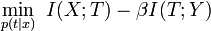
where  are the mutual information between
  and
and  respectively, and
  is a Lagrange multiplier.
Gaussian information bottleneck[edit]
A relatively simple application of the information bottleneck is to Gaussian variates and this has some semblance to a least squares reduced rank or canonical correlation [2]. Assume  are jointly multivariate zero mean normal vectors with covariances
  and is a compressed version of
  which must maintain a given value of mutual information with
  . It can be shown that the optimum is a normal vector consisting of linear combinations of the elements of
  where matrix
  has orthogonal rows.
The projection matrix in fact contains  rows selected from the weighted left eigenvectors of the singular value decomposition of the following matrix (generally asymmetric)

Define the singular value decomposition

and the critical values
then the number of active eigenvectors in the projection, or order of approximation, is given by

And we finally get
![A=[ w_1 U_1 , \dots , w_M U_M ]^T](http://upload.wikimedia.org/math/9/9/a/99ade49350ea3fa3d1049e68b91d55c4.png)
In which the weights are given by
where 
Applying the Gaussian information bottleneck on time series, one gets optimal predictive coding. This procedure is formally equivalent to linear Slow Feature Analysis [3]. Optimal temporal structures in linear dynamic systems can be revealed in the so-called past-future information bottleneck [4].
Data clustering using the information bottleneck[edit]
This application of the bottleneck method to non-Gaussian sampled data is described in [4] by Tishby et. el. The concept, as treated there, is not without complication as there are two independent phases in the exercise: firstly estimation of the unknown parent probability densities from which the data samples are drawn and secondly the use of these densities within the information theoretic framework of the bottleneck.
Density estimation[edit]
Since the bottleneck method is framed in probabilistic rather than statistical terms, we first need to estimate the underlying probability density at the sample points  . This is a well known problem with a number of solutions described by Silverman in [5]. In the present method, joint probabilities of the samples are found by use of a Markov transition matrix method and this has some mathematical synergy with the bottleneck method itself.
Define an arbitrarily increasing distance metric  between all sample pairs and distance matrix
  . Then compute transition probabilities between sample pairs
  for some
  . Treating samples as states, and a normalised version of
  as a Markov state transition probability matrix, the vector of probabilities of the ‘states’ after
  steps, conditioned on the initial state
  , is
, is  . We are here interested only in the equilibrium probability vector
  given, in the usual way, by the dominant eigenvector of matrix which is independent of the initialising vector . This Markov transition method establishes a probability at the sample points which is claimed to be proportional to the probabilities densities there.
Other interpretations of the use of the eigenvalues of distance matrix  are discussed in [6].
Clusters[edit]
In the following soft clustering example, the reference vector contains sample categories and the joint probability  is assumed known. A soft cluster
  is defined by its probability distribution over the data samples
  . In [1] Tishby et al. present the following iterative set of equations to determine the clusters which are ultimately a generalization of the Blahut-Arimoto algorithm, developed in rate distortion theory. The application of this type of algorithm in neural networks appears to originate in entropy arguments arising in application of Gibbs Distributions in deterministic annealing [7].
![\begin{cases} p(c|x)=Kp(c) \exp \Big( -\beta\,D^{KL} \Big[ p(y|x) \,|| \, p(y| c)\Big ] \Big)\\ p(y| c)=\textstyle \sum_x p(y|x)p( c | x) p(x) \big / p(c) \\ p(c) = \textstyle \sum_x p(c | x) p(x) \\ \end{cases}](http://upload.wikimedia.org/math/1/e/2/1e2fbfb1b963166cd0f7a60bd157f8fb.png)
The function of each line of the iteration is expanded as follows.
Line 1: This is a matrix valued set of conditional probabilities
![A_{i,j} = p(c_i | x_j )=Kp(c_i) \exp \Big( -\beta\,D^{KL} \Big[ p(y|x_j) \,|| \, p(y| c_i)\Big ] \Big)](http://upload.wikimedia.org/math/f/1/5/f152c3dae64059452ae85f0ed5eb2b27.png)
The Kullback–Leibler distance  between the vectors generated by the sample data
  and those generated by its reduced information proxy
  is applied to assess the fidelity of the compressed vector with respect to the reference (or categorical) data in accordance with the fundamental bottleneck equation.
  is the Kullback Leibler distance between distributions
and  is a scalar normalization. The weighting by the negative exponent of the distance means that prior cluster probabilities are downweighted in line 1 when the Kullback Liebler distance is large, thus successful clusters grow in probability while unsuccessful ones decay.
Line 2: This is a second matrix-valued set of conditional probabilities. The steps in deriving it are as follows. We have, by definition

where the Bayes identities  are used.
Line 3: this line finds the marginal distribution of the clusters

This is also a standard result.
Further inputs to the algorithm are the marginal sample distribution  which has already been determined by the dominant eigenvector of and the matrix valued Kullback Leibler distance function
![D_{i,j}^{KL}=D^{KL} \Big[ p(y|x_j) \,|| \, p(y| c_i)\Big ] \Big)](http://upload.wikimedia.org/math/e/e/8/ee821541e6604ed2bc7f9113eec967af.png)
derived from the sample spacings and transition probabilities.
The matrix  can be initialised randomly or as a reasonable guess, while matrix
  needs no prior values. Although the algorithm is converging, multiple minima may exist which need some action to resolve. Further details, including hard clustering methods, are found in [5].
Defining decision contours[edit]
To categorize a new sample  external to the training set , apply the previous distance metric to find the transition probabilities between and all samples in
  ,
,  with
with  a normalisation. Secondly apply the last two lines of the 3-line algorithm to get cluster, and conditional category probabilities.

Finally we have

Parameter  must be kept under close supervision since, as it is increased from zero, increasing numbers of features, in the category probability space, snap into focus at certain critical thresholds.
An example[edit]
The following case examines clustering in a four quadrant multiplier with random inputs  and two categories of output,
 , generated by
  . This function has the property that there are two spatially separated clusters for each category and so it demonstrates that the method can handle such distributions.
20 samples are taken, uniformly distributed on the square ![[-1,1]^2 \,](http://upload.wikimedia.org/math/e/8/a/e8a1ced319404e9fdb4c0785308c43ad.png) . The number of clusters used beyond the number of categories, two in this case, has little effect on performance and the results are shown for two clusters using parameters
. The number of clusters used beyond the number of categories, two in this case, has little effect on performance and the results are shown for two clusters using parameters  .
.
The distance function is  where
where 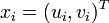 while the conditional distribution
  is a 2 × 20 matrix
and zero elsewhere.
The summation in line 2 is only incorporates two values representing the training values of +1 or −1 but nevertheless seems to work quite well. Five iterations of the equations were used. The figure shows the locations of the twenty samples with '0' representing Y = 1 and 'x' representing Y = −1. The contour at the unity likelihood ratio level is shown,
as a new sample is scanned over the square. Theoretically the contour should align with the  and
and  coordinates but for such small sample numbers they have instead followed the spurious clusterings of the sample points.
Neural network/fuzzy logic analogies[edit]
There is some analogy between this algorithm and a neural network with a single hidden layer. The internal nodes are represented by the clusters  and the first and second layers of network weights are the conditional probabilities
  and
and  respectively. However, unlike a standard neural network, the present algorithm relies entirely on probabilities as inputs rather than the sample values themselves while internal and output values are all conditional probability density distributions. Nonlinear functions are encapsulated in distance metric
  (or influence functions/radial basis functions) and transition probabilities instead of sigmoid functions. The Blahut-Arimoto three-line algorithm is seen to converge rapidly, often in tens of iterations, and by varying ,
  and and the cardinality of the clusters, various levels of focus on data features can be achieved.
The statistical soft clustering definition has some overlap with the verbal fuzzy membership concept of fuzzy logic.
Bibliography[edit]
[1] N. Tishby, F.C. Pereira, and W. Bialek: “The Information Bottleneck method”. The 37th annual Allerton Conference on Communication, Control, and Computing, Sep 1999: pp. 368–377
[2] G. Chechik, A Globerson, N. Tishby and Y. Weiss: “Information Bottleneck for Gaussian Variables”. Journal of Machine Learning Research 6, Jan 2005, pp. 165–188
[3] F. Creutzig, H. Sprekeler: Predictive Coding and the Slowness Principle: an Information-Theoretic Approach, 2008, Neural Computation 20(4): 1026–1041
[4] F. Creutzig, A. Globerson, N. Tishby: Past-future information bottleneck in dynamical systems, 2009, Physical Review E 79, 041925
[5] N Tishby, N Slonim: “Data clustering by Markovian Relaxation and the Information Bottleneck Method”, Neural Information Processing Systems (NIPS) 2000, pp. 640–646
[6] B.W. Silverman: “Density Estimation for Statistical Data Analysis”, Chapman and Hall, 1986.
[7] N. Slonim, N. Tishby: "Document Clustering using Word Clusters via the Information Bottleneck Method", SIGIR 2000, pp. 208–215
[8] Y. Weiss: "Segmentation using eigenvectors: a unifying view", Proceedings IEEE International Conference on Computer Vision 1999, pp. 975–982
[9] D. J. Miller, A. V. Rao, K. Rose, A. Gersho: "An Information-theoretic Learning Algorithm for Neural Network Classification". NIPS 1995: pp. 591–597
[10] P. Harremoes and N. Tishby "The Information Bottleneck Revisited or How to Choose a Good Distortion Measure". In proceedings of the International Symposium on Information Theory (ISIT) 2007
See also[edit]
External links[edit]